[Could not find the bibliography file(s)

I wrote a post a while ago with my tips for people that are starting off a physics degree. Just after I published it a friend and fellow post graduate, Sam Cooper, pointed out to me that I made a fairly blaring omission in my summary of undergraduate physics. Vectors. I was going to sneak in an extra section but I had a think and figured that it actually deserved its own post, so here goes.

If you’ve done A-level physics I’m sure you’ve come across the idea of a scalar before. Scalars are essentially just numbers that are used to represent quantities. They are only able to represent the magnitude of a measure, or put simply how much of something there is. Vectors are mathematical objects that allow you to represent not only the amount of something there is, but the direction in which this measure is acting as well. These are incredibly useful and as a result of this they are used extensively throughout physics. In an undergraduate degree the most applicable use of vectors are most likely going to be in vector mechanics and electromagnetism. I’ll go through some applications at the end, but first some theory.

Vector Algebra

Most people are used to manipulating scalars in the form of algebra, but when we’re using vectors we need some slightly different rules for manipulating mathematical expressions. This is the field of vector algebra. Because of these different rules it’s common for vectors to symbolised differently in equations. The problem is that there isn’t a globally consistent way of doing it. In some texts vectors are represented by emboldening the symbols, such as $\mathbf{a}$ . Another way, and the way which I shall use in this post, is by placing an arrow across the top of the symbol $\vec{a}$ . Just for the sake of formality, I’m going to be working in a 3 dimensional Euclidean space, the basis vectors of which consist of 3 orthonormal components. This may sound difficult to understand, so it’s worth explaining what this actually means. An orthonormal basis means that you build your vectors from basis vectors of unit length in that space and that none of the basis vectors can be projected into any of the others; they are all at right angles to one another. The basis vectors of Euclidean space are generally represented as $\hat{i}$ . $\hat{j}$ and $\hat{k}$ . These vectors lie along the x, y and z axes respectively. They can be represented in vector notation like so.

(1) $\begin{equation*} \hat{i} = \begin{pmatrix} 1 \\ 0 \\ 0 \end{pmatrix}\quad \hat{j} = \begin{pmatrix} 0 \\ 1 \\ 0 \end{pmatrix}\quad \hat{k} = \begin{pmatrix} 0 \\ 0 \\ 1 \end{pmatrix} \end{equation*}$

Now that we have correctly defined the basis, we can begin to make up our own vectors from these basis vectors. We do this by writing down how much of each basis vector we want. So let’s say for example we have a point, which we shall call $\vec{r}$ , which is at $x = 2$ , $y = 3$ and $z = 5$ . To express where this point is in 3D space we need to add together the right combination of basis vectors. We know that the basis vector $\hat{i}$ is in the positive $x$ direction and is a unit vector, so it represents +1 in the $x$ direction. The same reasoning goes for $\hat{j}$ in the $y$ direction and $\hat{k}$ in the $z$ direction. This means that we can represent the vector $\vec{r}$ like so:

(2) $\begin{equation*} \vec{r} = 2 \hat{i} + 3 \hat{j} + 5 \hat{k} \end{equation*}$

This vector can be illustrated schematically like so:

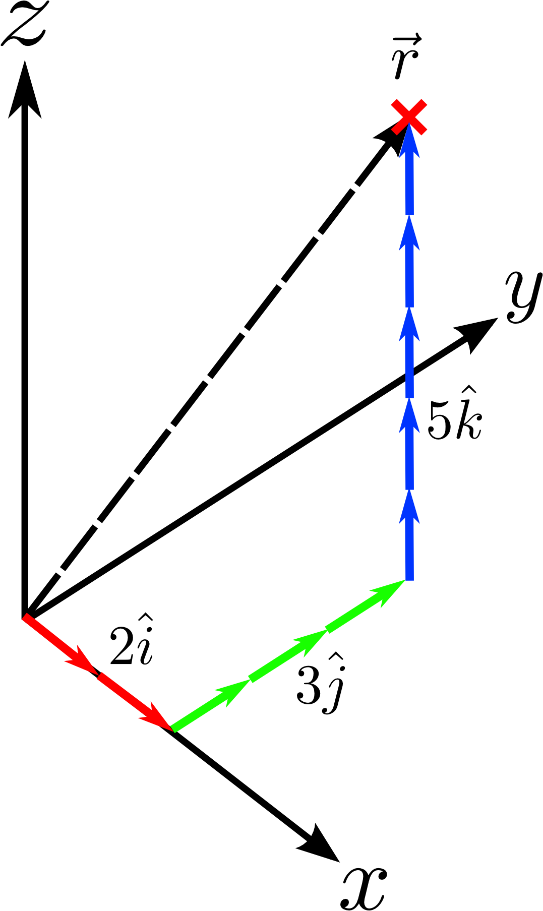
Vectors are made up from the basis vectors of a given space. In this example the vector $\vec{r}$ is made up of $2 \hat{i}$ (red), $3 \hat{j}$ (green) and $5 \hat{k}$ (blue). The black dashed line shows the resultant vector.

It can be a bit cumbersome using this notation all the way through the problem, so there’s an easy alternative. If we assume that all the vectors in a given problem use this same set of basis vectors we can also represent in short hand like so:

(3) $\begin{equation*} \vec{r} = \begin{pmatrix} 2 \\ 3 \\ 5 \end{pmatrix} \end{equation*}$

The same basis is necessary as in this notation there is nothing explicitly stating the basis. If in doubt just revert back to the long hand notation, shown in equation 2, as it leaves little room for ambiguity.

Vector Addition and Subtraction

Now that we have established the structure of a vector we can start to work with them. The first operation you should know, as with normal algebra, is addition and subtraction. Let’s say we have two vectors and we want to add them together:

(4) $\begin{equation*} \vec{r}_1 = \begin{pmatrix} 2 \\ 3 \\ 5 \end{pmatrix} \quad \vec{r}_2 = \begin{pmatrix} 1 \\ 3 \\ 7 \end{pmatrix} \quad \vec{r}_1 + \vec{r}_2 =\ ? \end{equation*}$

What we are essentially going to do here is once again decompose these vectors into the amounts of their basis vectors and add them all up. I’ll do this in long hand notation for clarity:

(5) $\begin{align*} \vec{r}_3 =\ \vec{r}_1 + \vec{r}_2\notag &=\ (2\hat{i} + 3\hat{j} + 5 \hat{k}) + (\hat{i} + 3\hat{j} + 7\hat{k})\\\notag &=\ (2 + 1)\hat{i} + (3 + 3)\hat{j} + (5 + 7)\hat{k}\\\notag &=\ 3\hat{i} + 6\hat{j} + 12\hat{k} \end{align*}$

The same methodology applies if you want to subtract a vector from another, just instead of adding the components together we take one set away from the other:

(6) $\begin{align*} \vec{r}_4 =\ \vec{r}_1 - \vec{r}_2\notag &=\ (2\hat{i} + 3\hat{j} + 5 \hat{k}) - (\hat{i} + 3\hat{j} + 7\hat{k})\\\notag &=\ (2 - 1)\hat{i} + (3 - 3)\hat{j} + (5 - 7)\hat{k}\\\notag &=\ \hat{i} - 2\hat{k} \end{align*}$

You should note here that the resulting vector has a negative contribution of $\hat{k}$ . It’s also worth nothing that the $\hat{j}$ is missing. This is because the resulting vector contains of $\hat{j} \times 0 = 0$ , so there’s no need to write that term down in this case.

The Magnitude of a Vector

It’s at this point convenient to introduce a new concept. When calculating things it’s often useful to work out the magnitude of something. With scalars this is simple as they are already the magnitude of the quantity they are intended to represent. However, there’s a small amount of calculation required to attain this information from a vector. This measure is called the magnitude, or Euclidean norm, of a vector. This calculation gives us the actual length of the vector and disregards the direction information. We can calculate it by adding up the square of all the components of a vector and then taking the square root, like so:

(7) $\begin{equation*} |\vec{X}| = \sqrt{x_1^2 + \cdots + x_N^2} \end{equation*}$

You’ll notice that the notation for the magnitude of a vector is the symbol for the vector with pipes placed around it $|\vec{X}|$ . This convention is actually fairly universal, so it should be easy to spot if you look out for the pipes on worksheets and textbooks. Just as an example, I’ll calculate the norm of $\vec{r}_1$ and $\vec{r}_2$ :

(8) $\begin{align*} |\vec{r}_1|\ &= \sqrt{2^2 + 3^2 + 5^2} = \sqrt{4 + 9 + 25} = \sqrt{38} = 6.16 \\ |\vec{r}_2|\ &= \sqrt{1^2 + 3^2 + 7^2} = \sqrt{1 + 9 + 49} = \sqrt{59} = 7.68 \end{align*}$

Vector Multiplication

This is where vectors get interesting. When working with scalars there is a single way to multiply two numbers together. The resulting answer is simply the product of the two numbers. In vector algebra however there are two different ways to multiply vectors, the dot product and the cross product. The dot product, or scalar product, of two vectors produces a scalar and can be thought of as the amount of one vector which is projected onto the other. In general, this is defined as:

(9) $\begin{equation*} \vec{X} \cdot \vec{Y}\ =\ |\vec{X}| |\vec{Y}| \cos(\theta) \end{equation*}$

where $\vec{X}$ and $\vec{Y}$ are two arbitrary vectors and $\theta$ is the angle between them if they are placed tail to tail. It’s worth noting at this point that vectors that are orthogonal and orthonormal, such as our basis vectors, will have a dot product of 0, as by very definition there will be no component of one projected onto the other. Using geometrical arguments we can see that in general the dot product of two vectors is also given by:

(10) $\begin{equation*} \vec{X}\cdot\vec{Y}\ =\ \sum^N x_i\ y_i \end{equation*}$

where $x_i$ and $y_i$ are the $i^\text{th}$ component of the $\vec{X}$ and $\vec{Y}$ vectors respectively. The other way of calculating the product of two vectors is called cross product, or the vector product, so called because it produces a vector. If we once again place the two vectors end to end we produce a hyperplane with one lower dimension that the space. In this case we create a 2D plane with the two vectors. The cross product produces a vector that is normal to this 2D plane, and hence orthogonal to both vectors original vectors. The cross product is defined as:

(11) $\begin{equation*} \vec{X} \times \vec{Y}\ =\ |\vec{X}||\vec{Y}| \sin \theta \hat{n} \end{equation*}$

where $\vec{X}$ and $\vec{Y}$ are the vectors to be operated on, $\theta$ is the angle between them and $\hat{n}$ is the unit vector that is normal to $\vec{X}$ and $\vec{Y}$ . Working all of these out can be quite time consuming, but if you’re comfortable with some basic matrix manipulation there’s a much easier way to work this out. Let’s adopt a $3 \times 3$ matrix and populate it with the basis vectors on the first row, the corresponding components of the first vector on the second row and the corresponding components of the second vector on the first row. It should look a little something like this:

(12) $\begin{equation*} \begin{pmatrix} \hat{i} & \hat{j} & \hat{k} \\ x_i & x_j & x_k \\ y_i & y_j & y_k \\ \end{pmatrix} \end{equation*}$

Now that we’ve constructed this matrix, if we take the determinant of this matrix we find that it produces a vector, which just happens to be the cross product. We can do this like so:

(13) $\begin{align*} \vec{X} \times \vec{Y}\ &=\ \begin{vmatrix} \hat{i} & \hat{j} & \hat{k} \\ x_i & x_j & x_k \\ y_i & y_j & y_k \\ \end{vmatrix} \\ &=\ \hat{i} (x_j y_k - x_k y_j)\ -\ \hat{j} (x_i y_k - x_k y_i)\ +\ \hat{k} (x_i y_j - x_j y_i) \end{align*}$

Once again as an example I shall find the cross product of $\vec{r}_1$ and $\vec{r}_2$ :

(14) $\begin{align*} \vec{r}_5\ =\ \vec{r}_1 \times \vec{r}_2\ &=\ \begin{vmatrix} \hat{i} & \hat{j} & \hat{k} \\ 2 & 3 & 5 \\ 1 & 3 & 7 \\ \end{vmatrix} \\ &=\ \hat{i} (3 \times 7 - 5 \times 3)\ -\ \hat{j} (2 \times 7 - 5 \times 1)\ +\ \hat{k} (2 \times 3 - 3 \times 1) \\ &=\ 6\hat{i} - 9\hat{j} + 3\hat{k}\ \end{align*}$

We stated before that any vector that results from the cross product of two vectors should itself be orthogonal to the other two vectors. We can verify this by taking the dot product of this derived vector $\vec{r}_5$ with $\vec{r}_1$ and $\vec{r}_2$ . If the vectors are orthogonal, the dot products should both come back as zero:

(15) $\begin{align*} \vec{r}_1 \cdot \vec{r}_5\ &=\ (2 \times 6) - (3 \times 9) + (5 \times 3) = 12 - 27 + 15 = 0\\ \notag \vec{r}_2 \cdot \vec{r}_5\ &=\ (1 \times 6) - (3 \times 9) + (7 \times 3) = 6 - 27 + 21 = 0\\ \notag \end{align*}$

Scalar and Vector Triple Product

There are also multiple ways of multiplying together three vectors. Since the dot product of two vectors results in a scalar, any further products involving this result is simply falls under normal rules for multiplication. However, the result of the cross product of two vectors results in another vector, so we can take this further. What about if we take the dot product of this with a third vector? This is known as the scalar triple product and is expressed as [?]:

(16) $\begin{equation*} \vec{a} \cdot (\vec{b} \times \vec{c}) \end{equation*}$

You can think of the result of this, ignoring the sign resulting from the initial vectors, as being the volume of a parallelepiped formed by the 3 originating vectors. If, like me, you’d never heard of this particular shape when you started I’ve included a link to the Wikipedia article. There are some interesting properties of this result that you may well need to know for a maths module. Firstly, the whole equation is completely invariant under circular shift. This just means that if we shift all the operands left or right in the equation we still get exactly the same answer [?]:

(17) $\begin{equation*} \vec{a} \cdot (\vec{b} \times \vec{c})\ =\ \vec{b} \cdot (\vec{c} \times \vec{a})\ =\ \vec{c} \cdot (\vec{a} \times \vec{b}) \end{equation*}$

Another property worth noting is that swapping around any two of the operands results in negating the triple product; changing the sign:

(18) $\begin{align*} \vec{a} \cdot (\vec{b} \times \vec{c})\ &=\ -\ \vec{b} \cdot (\vec{a} \times \vec{c})\notag\\ \vec{a} \cdot (\vec{b} \times \vec{c})\ &=\ -\ \vec{a} \cdot (\vec{c} \times \vec{b})\notag\\ \vec{a} \cdot (\vec{b} \times \vec{c})\ &=\ -\ \vec{c} \cdot (\vec{b} \times \vec{a})\notag\\ \end{align*}$

One final property that will come in useful later is that you can calculate the triple product by taking the determinant of a matrix containing those three vectors [?]:

(19) $\begin{equation*} \vec{a} \cdot (\vec{b} \times \vec{c})\ =\ \begin{vmatrix} a_1 & a_2 & a_3 \\ b_1 & b_2 & b_3 \\ c_1 & c_2 & c_3 \end{vmatrix}\ =\ a_1 (b_2 c_3 - b_3 c_2)\ -\ a_2 (b_2 c_3 - b_3 c_1)\ +\ a_3 (b_1 c_2 - b_2 c_1) \end{equation*}$

What about if we want to take the cross product of the cross product? This is called the vector triple product, and it’s defined as:

(20) $\begin{equation*} \vec{a} \times (\vec{b} \times \vec{c}) \end{equation*}$

By this definition, this useful relationship also holds [?]:

(21) $\begin{equation*} \vec{a} \times (\vec{b} \times \vec{c})\ =\ \vec{b}(\vec{a} \cdot \vec{c}) - \vec{c} (\vec{a} \cdot \vec{b}) \end{equation*}$

As we said before, the cross product is an anti-commutative operation. This means that you cannot change the two operands around and get the same answer, as we can with normal multiplication. We can use this to our advantage to define equivalent expressions, such as:

(22) $\begin{equation*} \vec{a} \times (\vec{b} \times \vec{c})\ =\ -\ (\vec{b} \times \vec{c}) \times \vec{a}\ =\ \vec{b}(\vec{a} \cdot \vec{c}) - \vec{c} (\vec{a} \cdot \vec{b}) \end{equation*}$

Vector Calculus

Up until this point we’ve studied vectors and how they’re exceedingly useful in a variety of applications in both mathematics and physics. However, in physics especially, studying steady state problems are particularly dull and are generally considered ‘trivial solutions’ to the governing equations of a system. We’re a lot more interested in dynamical systems that vary in time. For scalars we can study dynamical problems using calculus. The same is true when studying vectors, where we can use vector calculus. These operators are used when operating mathematical constructs called fields. During a degree you’ll most likely come across two different types of field, scalar fields and vector fields. A scalar field is a method of representing a given space by placing a number at every point a given space which represents a quantity. They can represent anything from density to electric fields. A vector field is very similar, but instead of placing a scalar at every point, you replace it with a vector. This is useful in disciplines such as fluid mechanics for representing the flow of a fluid. I’ll just go over the operators you can use

Gradient

The gradient or grad operator, signified as a nabla symbol $\nabla$ , allows the calculation of the gradient of a field. Just as the derivative calculates the gradient of a scalar function along one degree of freedom, the grad operator calculates the the gradient of every degree of freedom for a given field at the same time and returns the result as a vector. The grad operator for 3D euclidean space is defined as:

(23) $\begin{equation*} \vec{\nabla}\ =\ \left( \frac{\partial}{\partial x},\ \frac{\partial}{\partial y},\ \frac{\partial}{\partial z} \right) \end{equation*}$

As an example, let’s say that we have a function $f(x, y, z)\ =\ 3x^2 - 4x^3y^2 + 8z^5$ . Now let’s say that we apply the grad operator to this function:

(24) $\begin{equation*} \vec{\nabla} f(x, y, z)\ =\ \left( \frac{\partial f}{\partial x},\ \frac{\partial f}{\partial y},\ \frac{\partial f}{\partial z} \right)\ =\ \begin{pmatrix} 6x - 12x^2 \\ 8y \\ 40z^4 \end{pmatrix} \end{equation*}$

Divergence

The divergence or div operator is the result of taking the scalar product of the grad operator $\nabla$ with a vector field $\vec{a}$ , meaning that $\bf{div} \vec{a} = \vec{\nabla} \cdot \vec{a}$ . Physically, this can be thought of as the flow of the field into or out of an arbitrary point in the field. The number that comes out is a direct indicator of the flux flowing out of or in to the point. The sign of the resulting number also indicates the direction of the flow, with a negative number indicating a divergent flow where the field is flowing out of a point and a positive number indicating convergent flow where the field is flowing towards a point. This can also be described as a source or a sink respectively. For 3D Euclidean space, div is defined as:

(25) $\begin{equation*} \bf{div}\ \vec{a}\ =\ \vec{\nabla} \cdot \vec{a}\ =\ \frac{\partial a_1}{\partial x} + \frac{\partial a_2}{\partial y} + \frac{\partial a_3}{\partial z} \end{equation*}$

So, if we adopt the result of the previous example such that $\vec{a} = (6x - 12x^2)\hat{i} + 8y\hat{j} + 40z^4\hat{k}$ . If we now attempt to take the div of $\vec{a}$ , we get:

(26) $\begin{equation*} \vec{\nabla} \cdot \vec{a}\ =\ 6 - 24x + 8 - 120z^3\ = 14 - 24x - 120z^3 \end{equation*}$

We can now substitute in coordinates for this field to find out if the field is divergent at a given point. Let’s just for the sake of argument use $x = 2, y = 3$ and $z = 5$ . This yields a value of $\vec{\nabla} \cdot \vec{a} (2, 3, 5) = 14 - 48 - 600 = -638$ . This indicates that at the coordinates we specified, the field is strongly convergent and the point is acting as an effective sink.

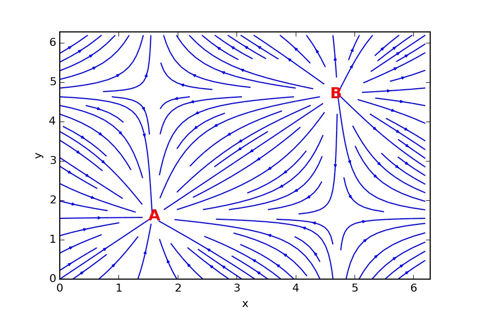
This figure shows a vector field with two points annotated. A shows a point of high divergence, where the arrows are flowing away from a source. B shows a point of high convergence, where the arrows flowing towards a sink.

This figure shows a vector field with two points annotated. A shows a point of high convergence, where the arrows are flowing towards a source. B shows a point of high divergence, where the arrows are flowing away from a source.

Curl

The final operator that I’m going to discuss in this post is the curl operator. This operator measures the infinitesimal rotation of a field at a given point in a vector field. This is essentially a measure of vorticity, the rotation of a flow. The curl of a field is defined as the cross product of the field with the grad operator, defined like so:

(27) $\begin{equation*} \bf{curl}\ \vec{a}\ =\ \vec{\nabla} \times \vec{a} \end{equation*}$

As previously we can use the determinant of a special crafted matrix to calculate the curl of a vector field $\vec{a}$ , like so:

(28) $\begin{align*} \bf{curl}\ \vec{a}\ &=\ \vec{\nabla} \times \vec{a}\ =\ \begin{vmatrix} \hat{i} & \hat{j} & \hat{k} \\ \frac{\partial}{\partial x} & \frac{\partial}{\partial y} & \frac{\partial}{\partial z} \\ a_1 & a_2 & a_3 \end{vmatrix} \notag\\ &\ =\ \left( \frac{\partial a_3}{\partial y} - \frac{\partial a_2}{\partial z} \right) \hat{i}\ +\ \left( \frac{\partial a_1}{\partial z} - \frac{\partial a_3}{\partial x} \right) \hat{j}\ +\ \left( \frac{\partial a_2}{\partial x} - \frac{\partial a_1}{\partial y} \right) \hat{k} \end{align*}$

Finally, let’s pluck a vector field out of the air and calculate its curl. $\vec{a} = 3z\hat{i} + 7x^2\hat{j} - 4y\hat{k}$ . If we now run this through the mathematics…

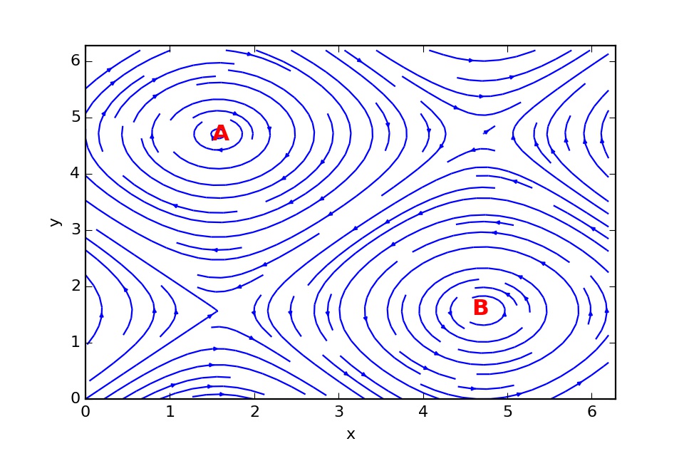
(29) $\begin{align*} \bf{curl}\ \vec{a}\ &=\ \vec{\nabla} \times \vec{a}\ =\ \begin{vmatrix} \hat{i} & \hat{j} & \hat{k} \\ \frac{\partial}{\partial x} & \frac{\partial}{\partial y} & \frac{\partial}{\partial z} \\ 3z & 7x^2 & -4y \end{vmatrix} \notag\\ &\ =\ (-4 - 0)\hat{i} + (3 - 0) \hat{j} + (14x - 0)\hat{k} \notag\\ &=\ -4\hat{i} + 3\hat{j} + 14x\hat{k} \end{align*}$

This figure shows another vector field. Points A and B show points of high vorticity, hence a large curl.

Applications

This concludes our whistle stop tour of vectors in physics. It’s at this point you’re probably wondering where you might be able to apply this knowledge of vectors. I’ve discussed the pure mathematics of it, but where can they be applied in physics problems? I’ll just go through some of them now.

Classical Mechanics

Classical mechanics is a discipline in physics that nearly relies entirely on vectors. This is why it’s often referred to as vector mechanics. It should come as no surprise that displacements of objects in physics problems are very easily represented using vectors. Not only this but vectors are ideally suited to representing the velocity and acceleration of an object. Another major use of vectors is the representation of forces in a classical system. Vectors are invaluable because they can not only represent the direction in which the force acts, but they can also represent the strength of the force. Many problems that you’ll be faced with in this topic will ask you to resolve forces. This means that you add all the forces being applied to an object together to come up with a net resultant force [?]. Once you’ve calculated this and, assuming that the force is constant, it’s a trivial matter to calculate the acceleration, velocity and position of an object over time.

Electromagnetism

When dealing with electromagnetic forces it’s often easy to lose sight of the fact that you’re actually dealing with the interaction of objects with the underlying electric and magnetic fields. Electric fields are easily represented as scalar fields. Using this representation we can perform all the operations mentioned above. Some of these operators are also used in the formulation of Maxwell’s equations, the fundamental equations of electromagnetism that have the power to describe not only the initial state and dynamical evolution of a given electromagnetic system, but they’re the root of some important proofs. One of the most iconic is the description of light as a coupled self-propagating electric and magnetic field. You can also perform integration within the framework of vector calculus. This is involved in the formulation and manipulation of Gauss’ equation. This equation allows the calculation of the electric field around a charge by performing a surface integral over a Gaussian surface surrounding the charge. Also using vector calculus you can calculate the magnetic field induced by a flowing current using a line integral. It’s probably fair to say that electromagnetism is probably the largest use of vector calculus that you will come across doing an undergraduate degree.

Fluid Mechanics

I’ve written extensively about fluid mechanics before in this post, this post and this post so I won’t bore you with the specifics, but just as in electromagnetism, fluid mechanics makes extensive use of vectors. The flow of a fluid is expressed as a vector field of velocities and the density of a fluid at each point can be expressed as a scalar field. Using these fields we can evolve a system using the governing equations of a given system. One of these is the momentum equation, known as the Navier-Stokes equation. This equation isn’t easily solvable, so studying the characteristics of the fluid using our operators can allow us to simplify it. The divergence operator can be used to see if the system we’re studying is an effective sink or source, allowing the characterisation of sink or source terms in our equations. The curl operator is a good measure of a system’s vorticity, allowing us to conveniently analyse flow characteristics; whether the system is in a laminar (slow, straight) regime, or a turbulent (fast, high vorticity) regime. With these fluid characteristics in mind, we can make meaningful simplifications to equations that make them easier to solve while retaining the physically significant terms.

Quantum Mechanics

At the moment you may find tackling the mathematical rigour of quantum mechanics a little daunting, and that’s because it is. It’s very difficult to represent the often obfuscated physics in an immediately obvious way. Vectors can actually help with this task. Quantum mechanics makes use of operators in order to attain physical quantities. Among them is the energy of a quantum system, provided by the Hamiltonian operator. This can be calculated using Schrödinger’s equation:

(30) $\begin{equation*} \left[ \frac{-\hbar^2}{2m} \nabla^2 + V(r) \right]\psi(r) = E \psi(r) \end{equation*}$

This is the time independent version of this equation. You can see that it makes use of the grad operator to attain its results. This important equation allows the calculation of the energies of all possible eigenstates of a particle. In some notations of quantum mechanics states of a particle can be represented as a vector. This vector contains probability amplitudes that express the superposition of states that constitute a given quantum system. This is true of various quantum operators such as energy and momentum. This representation holds true for any solvable quantum system, such as the infinite and quantum square well, known as the particle in a box, and the quantum harmonic oscillator. Although this is a less common use of vectors, its still worth noting.

Conclusion

That more or less sums up the basics you’ll probably need to know to get off to a good start with vectors at degree level. It’s worth stressing at this point that this post has focussed purely on 3D euclidean space. All of these operations are however completely applicable to any set of bases vectors. Probably the two most useful are cylindrical coordinates and spherical polar coordinates. Cylindrical coordinates adopt the $\hat{\theta}$ , $\hat{r}$ and $\hat{z}$ coordinates, which represent angle around a cylinder, radius outward from the origin and height from the origin respectively. Spherical polars adopt the $\hat{\rho}$ , $\hat{\phi}$ and $\hat{\theta}$ coordinates, which represent the radius outward from the origin, the angle around in the x-y plane between 0 and $2 \pi$ and elevation angle between $-\pi$ and $\pi$ . There are plenty of references out there and you can find plenty of examples out there of their use. As always I hope this post has been useful and if you notice anything amiss please do let me know and I’ll correct it ASAP. Until time, thanks for reading.

SAM MORRELL

An Undergrad Primer on Vectors

Vector Algebra

Vector Addition and Subtraction

The Magnitude of a Vector

Vector Multiplication

Scalar and Vector Triple Product

Vector Calculus

Gradient

Divergence

Curl

Applications

Classical Mechanics

Electromagnetism

Fluid Mechanics

Quantum Mechanics

Conclusion

Bibliography

Leave a Reply Cancel reply

Comments

Sorry, there are currently no comments for this artcle. Why not start a conversation?

About Me

Recent Posts

SAM MORRELL

An Undergrad Primer on Vectors

Vector Algebra

Vector Addition and Subtraction

The Magnitude of a Vector

Vector Multiplication

Scalar and Vector Triple Product

Vector Calculus

Gradient

Divergence

Curl

Applications

Classical Mechanics

Electromagnetism

Fluid Mechanics

Quantum Mechanics

Conclusion

Bibliography

Leave a Reply Cancel reply

Comments

Sorry, there are currently no comments for this artcle. Why not start a conversation?

About Me

Follow me

Recent Posts