Sam Morrell

In my last couple of posts I’ve been going through some of the basic principles of fluid mechanics. From some of the basic approximations that make the equation possible to analytically solve in this post, to some more specialised theory in the context of planetary systems in this post. In these posts we’ve been slowly working towards being able to understand the fluid mechanics used in modeling the atmospheres of exoplanets; which is just what I intend to do in this post. In order to improve current weather and climate models, scientists at both the UK Met Office and the University of Exeter have been collaborating to develop and test a new dynamical core for their global circulation model (GCM), called Unified Model (UM).

A Little Housekeeping…

Before introducing the equations that are solved by the dynamical core, it’s important to go over a few physical concepts that make an appearance in the formulation of the Unified Model.

The Geometry of the Problem

As we’re dealing explicitly with a planetary atmosphere, we can define our geometry with this in mind. If we define a set of orthogonal coordinates which we shall label $\hat{x}$ , $\hat{y}$ and $\hat{z}$ . These Cartesian axes rotate around the $\hat{z}$ axes with angular velocity $\vec{\Omega}$ . Around this coordinate system we now adopt a standard spherical coordinates system oriented such that the longitude $\lambda$ is in the $x-y$ plane and the latitude varies in $z$ .

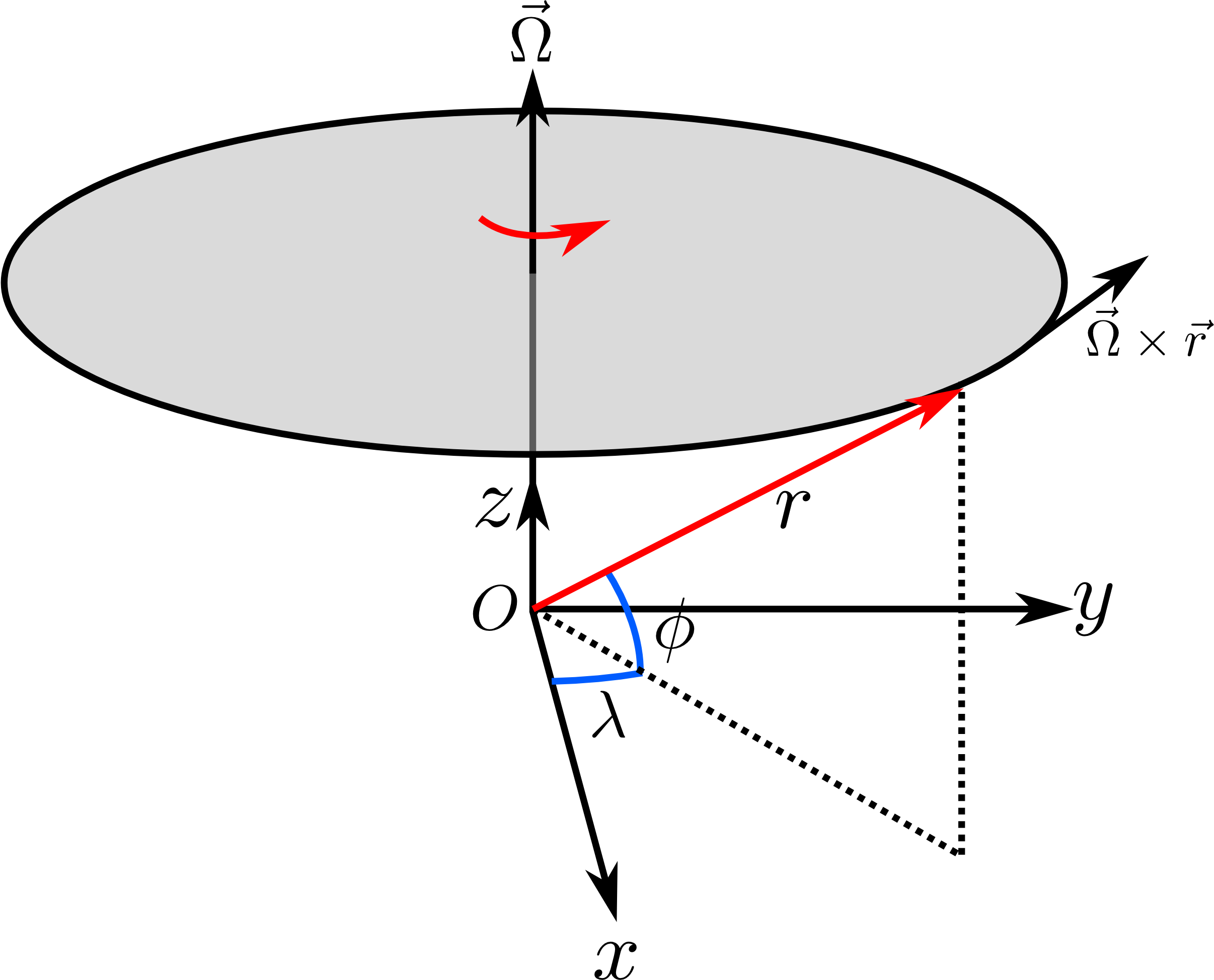
In line with astrophysical and meteorological convention we also define the the zonal and meridional direction. In reference to a planet, zonal refers to a direction following a circle of latitude around the globe in the west-east direction; whereas the meridional direction means ‘along a meridian’, or in a north-south direction.

Potential Temperature

As we’re dealing with the Lagrangian formulation of fluid mechanics, the dynamical equations refer to a parcel of fluid moving through the system. It’s for this reason that we define a temperature with this in mind. The potential temperature $\theta$ of a parcel of fluid held at pressure $p$ is the temperature that the parcel would acquire if it were adiabatically, meaning without any exchange of heat energy between it and its surroundings, brought to reference pressure $p_0$ . The potential temperature for air is given by:

(1) $\begin{equation*} \theta = T \left( \frac{p_0}{p} \right)^{R / C_p} \end{equation*}$

where $T$ is the absolute temperature of the parcel measured in K, $R$ is the gas constant for air and $C_p$ is the specific heat capacity of at constant pressure. In the context of meteorology, $p_0$ is usually taken as $1 \times 10^5$ Pa, or 1000 hPa.

Exner Function

The Exner function (or Exner Pressure) is a parameter appears a lot in atmospheric modeling. It is used as a non-dimensional measure of pressure. This may be preferable to normal measures of pressure as this parameter doesn’t introduce extra dimensions into equations. It is defined as:

(2) $\begin{equation*} \Pi = \left( \frac{p}{p_0} \right)^{R / C_p} = \frac{T}{\theta} \end{equation*}$

where $p_0$ is the puressure at the surface of the planet $R_d$ is the gas constant for dry air, $C_p$ is the heat capacity of dry air at constant pressure, $T$ is a the absolute temperature and $\theta$ is the potential temperature.

With these two parameters in place, we can simply define a relation between temperature and potential temperature simply becomes:

(3) $\begin{equation*} \theta = \frac{T}{\Pi} \end{equation*}$

The Fluid Mechanics

As with previous examples, we start of with our humble Navier-Stokes equation, written this time with an additional term that accounts for the effect of an imaginary centrifugal force, due to the rotation of the planet:

(4) $\begin{equation*} \frac{D \vec{u}}{D t} =\ - 2 \vec{\Omega} \times \vec{u}\ -\ \vec{\Omega} \times (\vec{\Omega} \times \vec{r})\ -\ \frac{1}{\rho} \nabla p\ +\ \vec{G} \end{equation*}$

in this formulation, $\vec{G}$ represents the force per unit mass and includes contributions from gravity, friction and electromagnetic forces. In the UM formulation, only friction and gravity are represented, thus:

$\vec{G}\ =\ - \nabla \Phi\ +\ \vec{S}^u$

where $\vec{S}^u$ is the frictional force per unit mass and $\Phi$ is the true gravitational potential. As a note, the negative of the gradient of $\Phi$ gives the acceleration due to distribution of mass. This contribution makes the equation of momentum become:

(5) $\begin{equation*} \frac{D \vec{u}}{D t} =\ - 2 \vec{\Omega} \times \vec{u}\ -\ \frac{1}{\rho}\nabla p\ -\ \nabla \Phi\ -\ \vec{\Omega} \times (\vec{\Omega} \times \vec{r}) + \vec{S}^u \end{equation*}$

Another factor that allows us to simplify the equation is the knowledge that the centrifugal term $-\ \vec{\Omega} \times (\vec{\Omega} \times \vec{r})$ can be written as the gradient of a centrifugal potential $\Omega^2 s^2 / 2$ , where $\vec{s}$ points perpendicularly outwards from the axis of rotation and has a a magnitude which is equal to the distance from it. With this knowledge, we can rewrite the centrifugal term as:

$\vec{\Omega} \times (\vec{\Omega} \times \vec{r}) = -\ \vec{\Omega} \times (\vec{\Omega} \times \vec{s}) =\ - \Omega^2 \vec{s} =\ -\nabla \frac{\Omega^2 s^2}{2}$

Hence, we can now define a quantity called the apparent gravitational potential $\Phi_a$ , which is defined as:

$\Phi_a = \Phi + \frac{1}{2} \Omega^2 s^2$

We can now operate the grad operator on the apparent gravitational potential to simply derive apparent gravity as:

$\nabla \Phi_a = g \hat{k}$

which is defined only in the direction pointing vertically outward from the surface of the planet. The variable $g$ can take varying forms, depending on the test case. We shall address these variations between cases later on in the post. Now our equation of motion simply becomes:

(6) $\begin{equation*} \frac{D \vec{u}}{D t} =\ - 2 \vec{\Omega} \times \vec{u} - \frac{1}{\rho} \nabla p - \vec{g} + S^{u} \end{equation*}$

It’s at this point it’s convenient to decompose this equation into its components, in order to solve numerically. We start by calculating the components of the Coriolis term:

(7) $\begin{align*} \vec{\Omega} \times \vec{u} &= \begin{vmatrix} \hat{i} & \hat{j} & \hat{k} \\ 0 & \Omega \sin \phi & \Omega \cos\phi \nonumber \\ u & v & w \\ \end{vmatrix} \\ &= ( 2 \Omega w \cos \phi\ -\ 2 \Omega v \sin \phi) \hat{i}\ +\ 2 \Omega u \sin \phi \hat{j}\ +\ 2 \Omega u \cos \phi \hat{k} \end{align*}$

Now that we have decomposed this cross product into the cartesian space, we need to finish the process by accounting for the fact that we’re dealing with an intrinsically curved, spherical geometry and that the local zonal, meridional and radial components, denoted as $\hat{i}$ , $\hat{j}$ and $\hat{k}$ respectively, will change direction as one moves across the surface. The terms that account for this in the decomposed equations are called metric terms and can be derived by isolating the components of the advective derivative, like so:

(8) $\begin{equation*} \frac{D \vec{u}}{Dt}\ =\ \frac{Du}{Dt}\hat{i}\ +\ \frac{Dv}{Dt}\hat{j}\ +\ \frac{Dw}{Dt}\hat{k} \end{equation*}$

For this geometry, this gives us the terms as:

(9) $\begin{align*} \frac{D \vec{u}}{D t}\ &=\ \hat{i}\left( \frac{Du}{Dt}\ -\ \frac{uv\tan \phi}{r}\ +\ \frac{uw}{r} \right) \nonumber \\ &+\ \hat{j} \left( \frac{Dv}{Dt}\ +\ \frac{u^2 \tan \phi}{r}\ +\ \frac{vw}{r} \right) \nonumber \\ &+\ \hat{k} \left( \frac{Dw}{Dt}\ -\ \frac{u^2\ +\ v^2}{r} \right) \end{align*}$

Given these two considerations we are now able to decompose the vectorial form of our momentum equation into its zonal, meridional and radial components, like so:

(10) $\begin{align*}\frac{Du}{Dt} &=\ -\ \frac{uw}{r}\ -\ 2 \Omega w \cos \phi\ +\ \frac{uv \tan \phi}{r}\ +\ 2 \Omega u \sin \phi \nonumber \\ &-\ \frac{1}{\rho r \cos \phi} \frac{\partial p}{\partial \lambda} + S^u \\ \frac{Dv}{Dt} &=\ -\ \frac{vw}{r}\ -\ \frac{u^2 \tan \phi}{r}\ -\ 2 \Omega u \sin \phi\ -\ \frac{1}{\rho r} \frac{\partial p}{\partial \phi} + S^v \\ \frac{Dw}{Dt} &=\ \frac{(u^2 + v^2)}{r}\ +\ 2 \Omega u \cos \phi\ -\ g\ -\ \frac{1}{\rho} \frac{\partial p}{\partial r} + S^w \end{align*}$

The advective derivative is given by:

(11) $\begin{equation*} \frac{D}{Dt}\ \equiv\ \frac{\partial}{\partial t}\ + \vec{u} \cdot \nabla\ \equiv\ \frac{\partial}{\partial t}\ +\ \frac{u}{r \cos \phi} \frac{\partial}{\partial \lambda}\ +\ \frac{v}{r} \frac{\partial}{\partial \phi}\ +\ w \frac{\partial}{\partial r} \end{equation*}$

The Equation of Continuity

In the system, we need to enforce mass conservation within the system. We do this using the continuity equation. This is usually expressed as $\nabla \cdot \vec{u} = 0$ for an incompressible fluid, however the more general case is:

(12) $\begin{equation*} \frac{\partial \rho}{\partial t}\ +\ \nabla \cdot (\rho \vec{u})\ =\ 0 \end{equation*}$

However, we can also express this equation in a more fundamental form involving the advective derivative:

(13) $\begin{equation*} \frac{D \rho}{D t}\ +\ \rho \nabla \cdot \vec{u}\ =\ 0 \end{equation*}$

Considering that we’re using polar coordinates, we can now derive the final equation that is used in the UM. This is:

(14) $\begin{equation*} \frac{D \rho}{D t}\ +\ \rho \left( \frac{1}{r \cos \phi} \left[ \frac{\partial u}{\partial \lambda}\ +\ \frac{\partial}{\partial \phi} (v \cos \phi) \right]\ +\ \frac{1}{r^2} \frac{\partial}{\partial r} \left[ r^2 w \right]\right)\ =\ 0 \end{equation*}$

The Thermodynamics

Now that we have considered the fluid mechanics which give us the flow of the material through the system, we must consider how this transports energy. We start of this endeavor by considering the first law of thermodynamics, which relates the change in internal energy of an arbitrary mass of the considered fluid $\delta U$ to the work done by the mass of fluid $\delta W$ . This relationship takes the form of:

(15) $\begin{equation*} \delta U = \delta Q - \delta W \end{equation*}$

in this equation we interpret $\delta Q$ as the total heating of the mass of fluid. This includes heat exchange from frictional dissipation, which is when energy transported through large scale convection is transferred to smaller and smaller energy scales until it is dissipated by frictional effects at molecular scales. Due to the entropic effects of this process, it’s irreversible. If the mass of the fluid has a pressure $p$ , and it’s volume $V$ reversibly changes, we can rewrite this as:

(16) $\begin{equation*} \delta U + p \delta V = \delta Q \end{equation*}$

In terms of quantities of these properties per unit mass, this becomes:

(17) $\begin{equation*} C_V \delta T + p \delta\alpha = \delta Q \end{equation*}$

where $\alpha = 1 / \rho$ . Given that in this equation $C_V$ is specific heat capacity at constant volume and $\alpha$ is a specific volume we can use the advective derivative to attain an expression that describes how the fluid is heated over time:

(18) $\begin{equation*} C_V \frac{D T}{D t} + p \frac{D \alpha}{D t} = \dot{Q} \end{equation*}$

in which $\dot{Q}$ is the rate of heating of a parcel of fluid per unit mass. If we now assume that the atmosphere is a perfect gas, where we can set $p \alpha = RT$ and $C_p - C_V = R$ we find the equation:

(19) $\begin{equation*} C_p \frac{D T}{D t} - \alpha \frac{D p}{D t} = \dot{Q} \end{equation*}$

We can now conveniently parameterise this expression using the potential temperature that we’ve used several times before in this post. Making the substitution gives us the simplified thermodynamic equation that is used in the UM:

(20) $\begin{equation*} \frac{D \theta}{D t} = \left( \frac{\theta}{T} \right) \frac{\dot{Q}}{C_p} \end{equation*}$

In this expression the non-dimensional $(\theta / T)$ term acts as a source term for the equation, which is then multiplied by the heating rate $\dot{Q}$ divided by $C_p$ .

Equation of State

For this model we shall assume that the atmosphere consists of dry air. In the operational model, atmospheric moisture is considered separately. In order to treat thermodynamics in the model, we choose to adopt the ideal gas law. The most well known version of this law is:

(21) $\begin{equation*} pV = nRT = N k_B T \end{equation*}$

In this case, it’s chosen to be represented in terms of density $\rho$ , like so:

(22) $\begin{equation*} p = \rho R T \end{equation*}$

In general, it’s preferable to represent variables of state in terms of dimensionless quantities. In this case we can represent pressure in the function as the Exner function and temperature in terms of the potential temperature. Substituting this in, and introducing $\kappa = R / C_p$ , we arrive at our equation of state for the Unified Model:

(23) $\begin{equation*} \Pi^{\frac{\kappa - 1}{\kappa}} \rho \theta = \frac{p_0}{\kappa C_p} \end{equation*}$

Parameterising the Pressure Gradient

Given that we’ve parameterised variables in the equation of state, it’s sensible to also adopt them for the pressure gradient terms in the equations of momentum. By substituting $\Pi$ for pressure, the pressure gradient term becomes:

(24) $\begin{equation*} \frac{1}{\rho} \frac{\partial p}{\partial X}\ =\ \frac{RT}{p} \frac{\partial p}{\partial X}\ =\ \frac{R \theta \Pi}{p} \frac{\partial p}{\partial X}\ =\ C_p \theta \frac{\partial \Pi}{\partial X} \end{equation*}$

where $X$ is a coordinate, either $\lambda$ , $\phi$ or $r$ . By substituting this relation into the equations of momentum we end up with the final equations of momentum, for zonal, meridional and vertical flow respectively:

(25) $\begin{align*} \frac{Du}{Dt} &=\ -\ \frac{uw}{r}\ -\ 2 \Omega w \cos \phi\ +\ \frac{uv \tan \phi}{r}\ +\ 2 \Omega u \sin \phi \nonumber \\ &-\ \frac{C_p \theta}{r \cos \phi} \frac{\partial \Pi}{\partial \lambda} + S^u \\ \frac{Dv}{Dt} &=\ -\ \frac{vw}{r}\ -\ \frac{u^2 \tan \phi}{r}\ -\ 2 \Omega u \sin \phi\ -\ \frac{C_p \theta}{r} \frac{\partial \Pi}{\partial \phi} + S^v \\ \frac{Dw}{Dt} &=\ \frac{(u^2 + v^2)}{r}\ +\ 2 \Omega u \cos \phi\ -\ g\ -\ C_p \theta \frac{\partial \Pi}{\partial r} + S^w \end{align*}$

Test Cases

Now that we have the set of equations that make up the dynamical core of the UM, a momentum equation for each coordinate, a continuity equation to ensure mass conservation, a thermodynamic energy equation which describes heating of the fluid and an equation of state which describes an idea gas, we can consider some test cases for which they are applicable. Considered in the research relating to this post are both terrestrial planets and hot Jupiters. Both of these cases are important to test due to Earth-like exoplanet climates and the dynamics of hot Jupiter atmospheres being very active research areas.

The main differentiation between test cases is the temperature profile and structure of the model atmosphere. In the following sections I will summarise some of the test cases that the UM has been subjected to. Each one has subtle differences in model, so if you want more detail refer to source materials in the references. In interpreting the results from these test cases it’s also useful to understand the concept of normalised pressure. This is effectively a vertical coordinate within the system and is defined as:

(26) $\begin{equation*} \sigma = \frac{p}{p_s} \end{equation*}$

where $p$ is the pressure at a given layer in the atmosphere, $p_s$ is the pressure at the surface, or lower boundary, of the model and $\sigma$ represents the normalised pressure. By definition, at the surface of the planet $\sigma = 1$ and at $p = 0$ , $\sigma = 0$ . This imposes the condition that $\dot{\sigma} = 0$ at both the top and bottom boundary. More generally, we can allow for an upper boundary condition to be set to a constant finite pressure $p_T$ using:

(27) $\begin{equation*} \sigma = \frac{p - p_T}{p_s - p_T} = \frac{p - p_T}{\pi} \end{equation*}$

with $\pi$ generally being defined in literature as the pressure difference between the top and bottom pressure of a model. Usefully, we can note that if the pressure at the upper boundary is 0, then this generalised form of the equation will become the equation for the special case we mentioned above. This coordinate system is useful as it allows the complex bottom boundary conditions that the orography of the planets surface would cause. However, there is no orography for these test cases.

You’ll recall that earlier on we discussed the thermodynamics of the model and we defined the heating rate $\dot{Q}$ . In the following cases the heating of the system is provided by radiative transfer. This is a achieved either by forcing to an atmospheric temperature profile or through Newtonian cooling. The heating rate is set by $\dot{Q}_\text{Newton}$ which can be represented as a function of prognostic variables which the code calculates:

(28) $\begin{equation*} \dot{Q}\ =\ \dot{Q}_\text{Newton}\ =\ -\ \Pi \left( \frac{\theta - \theta_\text{eq}}{\tau_\text{rad}} \right) \end{equation*}$

where $\tau_\text{rad}$ is the characteristic radiative or relaxation timescale and $\theta_\text{eq}$ is the equilibrium potential temperature, and can be attained from the equilibrium temperature profile $T_\text{eq}$ on the $i^\text{th}$ time-step using:

(29) $\begin{equation*} \theta^i_\text{eq}\ =\ \frac{T_\text{eq}}{\Pi^i} \end{equation*}$

The Held-Suarez Test

The Held-Suarez test, described in Held & Suarez (1994), is a simple global circulation test case developed in order to aid intercomparison of GCMs regardless of parameterisation or formulation differences. It’s main focus is testing the long term statistical properties of atmospheric circulation; making it particularly useful for climate codes, such as the UM, which are required to model decades in advance. In this case numerical stability and accuracy of the code is a priority. The equilibrium temperature profile for the test case is:

(30) $\begin{equation*} T_\text{eq} = \text{max} \left\{T_\text{stra}, T_\text{HS} \right\} \end{equation*}$

where $T_\text{stra} = 200$ K. $T_\text{HS}$ is given by:

(31) $\begin{equation*} T_\text{HS} = \left[ T_\text{surf} - \Delta T_\text{EP} \sin^2 \phi - \Delta T_z \ln \left( \frac{p}{p_0} \right) \cos^2 \phi \right] \left( \frac{p}{p_0}\right)^\kappa \end{equation*}$

where $T_\text{surf} = 315$ K, $\Delta T_\text{EP} = 60$ K, $\Delta T_z = 10$ K and $p_0 = 1 \times 10^5$ Pa. For this model, the radiative timescale $\tau_\text{rad}$ is modeled as:

(32) $\begin{equation*} \frac{1}{\tau_\text{rad}}\ =\ \frac{1}{\tau_\text{rad, d}}\ +\ \begin{cases} 0\ &\text{where}\ \sigma \leq \sigma_b \\ \left( \frac{1}{\tau_\text{rad,du}} - \frac{1}{\tau_\text{rad,d}} \right) \left( \frac{\sigma - \sigma_b}{1 - \sigma_b} \right) \cos^4 \phi\ &\text{where}\ \sigma > \sigma_b \end{cases} \end{equation*}$

where $\tau_\text{rad,d} = 40$ days, $\tau_\text{rad,u} = 4$ days and $\sigma_b =0.7$ , which is the sigma coordinate for the top of the surface friction boundary layer, the layer in which the dominant effect on wind damping is the friction of the planetary surface. This layer imposes frictional damping on a timescale $\tau_\text{fric}$ of:

(33) $\begin{equation*} \frac{1}{\tau_\text{fric}}\ = \begin{cases} 0\ &\text{where}\ \sigma \leq \sigma_b \\ \left( \frac{1}{\tau_\text{fric, f}} \right) \left( \frac{\sigma - \sigma_b}{1 - \sigma_b} \right) &\text{where}\ \sigma > \sigma_b \end{cases} \end{equation*}$

where $\tau_\text{fric, f} = 1$ day. Given this prescription the prognostic variables can then be time averaged and compared to other results as an intercomparison test for GCM validity. This test exists mainly because analytical tests, such as the Sod shock tube for advection in 1D, aren’t possible for complex flow like global circulation.

A Simple Earth-like Case Including a Stratosphere

This simple Earth-like test case is described in Menou & Rauscher (2009). This model bears a resemblance to the Held-Suarez test described above, however it can be considered a cruder version due to several simplifications. A prime example of this is the adoption of single values for $\tau_\text{rad} = 15$ days and $\tau_\text{fric} = 1$ day throughout the atmosphere, as opposed to the parameterisations used in the Held-Suarez model. This has the effect of bringing down the number of free parameters. One feature of this model is that the vertical equilibrium temperature profile is parameterised in such a way as to add an isothermal stratosphere. The equilibrium temperature profile $T_\text{eq}$ is given as:

(34) $\begin{equation*} T_\text{eq}\ =\ T_\text{vert}\ +\ \beta_\text{trop} \Delta T_\text{EP} \left( \frac{1}{3} - \sin^2 \phi \right) \end{equation*}$

where $\Delta T_\text{EP} = 60$ K is the equator-to-pole temperature difference and the vertical variation in equilibrium temperature $T_\text{vert}$ is given by:

(35) $\begin{equation*} T_\text{vert}\ = \begin{cases} T_\text{surf} - \Gamma_\text{trop} (z_\text{stra} + \frac{z - z_\text{stra}}{2}) \\ + \left( \left[ \frac{z - z_\text{stra}}{2} \right]^2 + \Delta T^2_\text{strat} \right) &\ \text{where}\ z \leq z_\text{stra} \\ T_\text{surf} - \Gamma_\text{trop} z_\text{stra}\ +\ \Delta T_\text{strat} &\ \text{where}\ z > z_\text{stra} \end{cases} \end{equation*}$

where $T_\text{surf} = 288$ K is the surface temperature of the modeled planet, $\Gamma_\text{trop} = 6.5 \times 10^{-8}$ K m $^{-1}$ is the lapse rate, which is the rate at which temperature decreases with increasing height in the atmosphere, and $\Delta T_\text{strat} = 2$ K, which acts as an offset to smooth transition from the troposphere to the isothermal stratosphere. The boundary between these two layers is called the tropopause and is defined in real and sigma vertical coordinates by $z_\text{stra}$ and $\sigma_\text{stra}$ respectively. Finally, $\beta_\text{trop}$ is a height-dependent damping factor applied to the troposphere in order gradually reduce the latitudinal and longitudinal temperature differential over the vertical extent of the troposphere. It is defined as:

(36) $\begin{equation*} \beta_\text{trop}\ = \begin{cases} \sin \frac{\pi (\sigma - \sigma_\text{stra})}{2 (1 - \sigma_\text{stra})} &\ \text{where}\ z \leq z_\text{stra}\ \text{or}\ \sigma \geq \sigma_\text{stra} \\ 0&\ \text{where}\ z > z_\text{stra}\ \text{or}\ \sigma < \sigma_\text{stra} \end{cases} \end{equation*}$

As opposed to the Held-Suarez test, which is meant to test the code, this test is designed to offer insight into model parametrisations and the accuracies thereof. Instead of being able to exactly reproduce the characteristics of Earth’s global circulation, as was the aim of the Held-Suarez test, it’s often far more useful to be able to reproduce the main qualitative features for a more general case. The main reason being that the atmospheric conditions on Earth are very well known so the models can be tweaked to fit the known conditions, however conditions on exoplanets aren’t so well constrained. Models need to be able to reliably reproduce global circulation for an atmosphere without a priori knowledge of its characteristics, such is the case on all planets outside of the Solar System.

A Tidally Locked Earth-like Case

In this theoretical model we adjust the rotation rate of the Earth-like planet so that a day is equal to one orbital period, $\Omega \rightarrow \frac{\Omega}{365}$ . This situation is known as tidal locking. In this regime the planet has a permanent day and night side and the wind is responsible for heat transport from the permanently radiated day side to the permanently dark night side. This introduces a steep longitudinal temperature gradient between the day and night sides of the planet. Importantly, this is generally an affect found in hot Jupiter planets, which have a very different atmospheric structure and heat transport regime. This model allows the code to be run in familiar conditions in an Earth-like atmosphere, while introducing aspects found in hot Jupiter atmospheres. Once again, the model takes inspiration from the Held-Suarez model, using the equation for equilibrium temperature profile with modifications to enforce a longitudinal temperature contrast and ‘hot spot’ at the subsolar point centred on the equator at a longitude of 180 $^\circ$ . It is given by:

(37) $\begin{equation*} T_\text{eq}\ =\ \text{max} \left\{ T_\text{stra}, T_\text{TLE} \right\} \end{equation*}$

where,

(38) $\begin{equation*} T_\text{TLE}\ =\ \left[ T_\text{surf} + \Delta T_\text{EP} \cos (\lambda - 180^\circ) \cos \phi - \Delta_z \ln \left( \frac{p}{p_0} \right) \cos^2 \phi \right] \left( \frac{p}{p_0} \right)^\kappa \end{equation*}$

All values that are present in the Held-Suarez model take the same value in this one. In this model it’s likely that significant flow over the pole will be present, so it’s necessary to add a sponge layer into the UM to damp vertical motion and improve model stability. As an example, the vertical velocity, with damping $R_w$ , is given by:

(39) $\begin{equation*} w^{t + \Delta t} = w^t + S_w - R_w \Delta t w^{t + \Delta T} \end{equation*}$

where $w^t$ and $w^{t + \Delta t}$ are the vertical velocities at the current and future timesteps respectively, $S_w$ is a source term and $\Delta t$ is the length of the timestep. The spatial extend of this damping coefficient is given by:

(40) $\begin{equation*} R_w\ = \begin{cases} C \left( \sin^2 \left( 0.5 \pi (\eta - \eta_s) \left( \frac{1.0}{1.0 - \eta_s} \right) \right) + \sin^{40} (\phi)\right) &\ \text{where}\ \eta \geq \eta_s \\ 0 &\ \text{where}\ \eta < \eta_s \end{cases} \end{equation*}$

where, given that there is no orography present on the surface, $\eta = z / H$ , $\eta_s = 0.75$ is the start height of the top level damping and $C = 0.05$ is a coefficient.

A Shallow Hot Jupiter Case

We now move away from Earth-like planets in favour of the another great focus of exoplanet research; hot Jupiters. Fundamentally, the atmospheres of hot Jupiters have very different circulation regime to terrestrial planets. A shallow hot Jupiter test case is laid out in Menou & Rauscher (2009). In this test case, the atmosphere is termed a shallow hot Jupiter as the atmosphere is only modeled down to $1 \times 10^5$ Pa. No account is made of atmosphere below this level. Despite this massive simplification, one clear advantage is that it is a direct extension of the Earth-like atmospheric model described earlier in the post. This allows easy comparison between the two circulation regimes. The vertical temperature profile $T_\text{vert}$ and tropospheric damping factor $\beta_\text{trop}$ remain mathematically the same as in the Earth-like case, however the equilibrium temperature profile $T_\text{eq}$ becomes:

(41) $\begin{equation*} T_\text{eq} = T_\text{vert} + \beta_\text{trop}\Delta T_\text{EP} \cos (\lambda = 180^\circ) \cos(\phi) \end{equation*}$

The radiative timescale $\tau_\text{rad}$ is once again set to $\pi / \Omega_p \sim 1.731$ days throughout the atmosphere. There are also simplifications made to the equations in the dynamical core, however we shall not detail that in this summary. Now that we have a shallow test case laid out for a hot Jupiter, what about the full hot Jupiter?

A Full Hot Jupiter Case

This test case is modeled after the commonly studied exoplanet, HD 209458b. This case is adapted from the one described in Heng (2011). This time the equilibrium temperature and relaxation profiles were modeled based on observations. In these profiles there’s a radiatively inactive region that reaches from $2.2 \times 10^7$ Pa to $1 \times 10^6$ Pa where $\tau_\text{rad} = \infty$ . Above this there’s a radiatively active region. As the exoplanet has a day- and night-side, two different equilibrium temperature profiles are required to model it. The temperature profile for the night side $T_\text{night}$ is given by:

(42) $\begin{equation*} T_\text{night}\ =\ \begin{cases} T^\prime_\text{night} |^{p_\text{high}} + 100\text{K} (1.0 - e^{-(\log(p) - \log(p_\text{high}))})&\ \text{where}\ p \geq p_\text{high} \\ \text{max} \left\{ T^\prime_\text{night} |^{p_\text{low}} \times e^{0.10 (\log (p) - \log(p_\text{low}))}, 250 \right\} &\ \text{where}\ p \geq p_\text{low} \\ T^\prime_\text{night} |^p &\ \text{otherwise} \end{cases} \end{equation*}$

and the temperature profile of the day side $T_\text{day}$ is given by:

(43) $\begin{equation*} T_\text{day}\ =\ \begin{cases} T^\prime_\text{day} |^{p_\text{high}} - 120\text{K} (1.0 - e^{-(\log(p) - \log(p_\text{high}))})&\ \text{where}\ p \geq p_\text{high} \\ \text{max} \left\{ T^\prime_\text{day} |^{p_\text{low}} \times e^{0.0150 (\log (p) - \log(p_\text{low}))}, 1000\right\} &\ \text{where}\ p \geq p_\text{low} \\ T^\prime_\text{day} |^p &\ \text{otherwise} \end{cases} \end{equation*}$

where $T_\text{day}$ and $T_\text{night}$ are the day and night side temperature profiles respectively, $T^\prime_\text{day}$ and $T^\prime_\text{night}$ are the polynomial fits to modeled temperature profiles and $p_\text{low}$ and $p_\text{high}$ are 100 and $1 \times 10^6$ Pa respectively. We then combine these two profiles together to create a temperature map of the planet using:

(44) $\begin{equation*} T_\text{eq}\ = \begin{cases} \left[ T^4_\text{night} + (T^4_\text{day} - T^4_\text{night}) \cos(\lambda - 180^\circ) \cos \phi \right]^\frac{1}{2} &\ \text{where}\ 90^\circ \leq \lambda \leq 270^\circ \\ T_\text{night} &\ \text{otherwise} \end{cases} \end{equation*}$

This is run using the full set of governing equations and, as with the tidally locked Earth-like case, a sponge layer is added in for numerical stability. The sponge layer is defined in the tidally locked Earth case, but for this we alter the parameters, taking a value of $\eta_s = 0.75$ for all cases, $C = 0.2$ for the deep and shallow equations, but $C = 0.15$ for the full equations.

In Conclusion

For this post I’ve been through some details of the formulation of the Met Office’s global circulation model, the Unified Model. These equations include the momentum equations, the equation of continuity, the thermodynamic equation for the system and finally the equation of state. Having gone through these core equations of the UM, we then go on to briefly summarise some test cases which the UM was subjected to. These ranged from simple, Earth-like cases to hot Jupiter cases. If you’d like more details on any of the cases I described to you the links to papers are down in the references, and if you’re interested I highly recommend checking them out. Until next time, I hope you enjoyed reading this long, drawn out post as much as I enjoyed researching and writing it. Until next time, thanks for reading.

References

Tags:

climate fluid mechanics Met model Office Physics unified

SAM MORRELL

Modeling Atmospheres with the Unified Model

A Little Housekeeping…

The Geometry of the Problem

Potential Temperature

Exner Function

The Fluid Mechanics

The Equation of Continuity

The Thermodynamics

Equation of State

Parameterising the Pressure Gradient

Test Cases

The Held-Suarez Test

A Simple Earth-like Case Including a Stratosphere

A Tidally Locked Earth-like Case

A Shallow Hot Jupiter Case

A Full Hot Jupiter Case

In Conclusion

References

Tags:

Leave a Reply Cancel reply

Comments

Sorry, there are currently no comments for this artcle. Why not start a conversation?

About Me

Recent Posts

SAM MORRELL

Modeling Atmospheres with the Unified Model

A Little Housekeeping…

The Geometry of the Problem

Potential Temperature

Exner Function

The Fluid Mechanics

The Equation of Continuity

The Thermodynamics

Equation of State

Parameterising the Pressure Gradient

Test Cases

The Held-Suarez Test

A Simple Earth-like Case Including a Stratosphere

A Tidally Locked Earth-like Case

A Shallow Hot Jupiter Case

A Full Hot Jupiter Case

In Conclusion

References

Tags:

You Might Also Like...

Chirp has a New Home

My Top Tips for Preparing for a Physics Degree

University is Over… for Now

The Fluid Mechanics of Planetary Atmospheres

Leave a Reply Cancel reply

Comments

Sorry, there are currently no comments for this artcle. Why not start a conversation?

About Me

Follow me

Recent Posts

References

- Held, I. M. & Suarez, M. J. (1994), ‘A Proposal for the Intercomparison of the Dynamical Cores of Atmospheric General Circulation Models’, Bull. Amer. Meteor. Soc. 75(10), 1825–1830.
- Menou, K. & Rauscher, E. (2009), ‘Atmospheric Circulation of Hot Jupiters: A Shallow Three-Dimensional Model’, 700, 887-897.
- Merlis, T. M. & Schneider, T. (2010), ‘Atmospheric Dynamics of Earth-Like Tidally Locked Aquaplanets’, Journal of Advances in Modeling Earth Systems 2(4)
- Heng, K.; Menou, K. & Phillipps, P. J. (2011), ‘Atmospheric circulation of tidally locked exoplanets: a suite of benchmark tests for dynamical solvers’, 413, 2380-2402.