At the moment I’m intently studying fluid mechanics for an exam on planetary science. As you may have guessed, the fluid mechanics in question is for modelling planetary atmospheres, but the mathematics is universally applicable. I’ve wanted to learn fluid mechanics for many years so I thought I’d just go through some of the basics and a few examples of fluid mechanics in action. Before we get started, I just want to say that it’s probably not as hard as you think it is. When you’ve got some of the fundamentals out of the way, there’s just a little mathematics and heaped helping of thermodynamics that should get us all the results we need. Without further ado, off we go on a breakneck tour of fluid mechanics.
The Momentum Equation
In classical mechanics, there’s a very famous equation that more or less everybody knows which describes how an object with mass  moves when a force is applied to it. This is so famous that it is given the name of Newton’s 2nd Law of Motion and is expressed as:
![\[\vec{F} = m \vec{a}\]](https://sammorrell.co.uk/wp-content/ql-cache/quicklatex.com-7130472f42a44629df163a23cf3554e5_l3.png "Rendered by QuickLaTeX.com")
All this equation states is that the force  you apply to an object makes the object you apply it to accelerate in the same direction as the force with an acceleration
  of the force divided by it’s mass. This applies excellently for a non-relativistic object, however it somewhat fails to describe a continuum of objects, like a liquid that has a force applied to it. This is where fluid mechanics comes in. In this case, the equation we use to describe the dynamics of a liquid is called the Navier-Stokes equation and we’re going to use it a lot. For an incompressible fluid, this can be expressed as:
![\[\rho \left( \frac{\partial \vec{v}}{\partial t} + \vec{u} \cdot \nabla \vec{u} \right) = \ - \nabla P + \rho \vec{g} + \mu \nabla^2 \vec{v}\]](https://sammorrell.co.uk/wp-content/ql-cache/quicklatex.com-8a89233565211bb76bfcae54157908ff_l3.png "Rendered by QuickLaTeX.com")
Initially, this equation may seem long and terrifying, but let’s take it apart and see how it works. Let’s say that we’re using the Lagrangian description of fluid mechanics, where we consider a parcel of material moving through the system and follow it. In this description we need to consider how the properties of the parcel change locally and in relation to the flow through the bulk fluid. Considering this mathematical details, the equation that describes a this system is:
![\[\rho \left( \underbrace{\frac{\partial \vec{v}}{\partial t}}_a + \underbrace{\vec{u} \cdot \nabla \vec{u}}_b \right) = \underbrace{\ - \nabla P}_c + \underbrace{\rho \vec{g}}_d + \underbrace{\mu \nabla^2 \vec{v}}_e\]](https://sammorrell.co.uk/wp-content/ql-cache/quicklatex.com-335bc9a7357eea4fffdd0dcb25aeb4d9_l3.png "Rendered by QuickLaTeX.com")
The terms in this equation each correspond to an important bit of physics:
- Local acceleration term: Describes how the flow accelerates locally in the packet of material.
- Inertial / non-linear term: Describes how the flow of a packet of material affects a property; in this case the flow itself.
- Pressure gradient term: This tells us the direction in which direction the pressure change is in.
- Gravity term: This introduces the effect of gravity into the system. For some systems, this isn’t important so we can just lose it.
- Viscosity term: This term describes how viscosity affects the system.
In the context of a rotating fluid, we can also add in another term to describe the affect of rotation on a fluid; which is particularly important in planetary and climate science. This is called the Coriolis term, and it’s given by:
![\[- 2 \vec{\Omega} \times \vec{u}\]](https://sammorrell.co.uk/wp-content/ql-cache/quicklatex.com-8108c09e1c0720c7508ad830cbd7ab18_l3.png "Rendered by QuickLaTeX.com")
where  is the rotation of the planet.
The Advective Derivative
Because it’s so useful, the terms on the left hand side of the Navier-Stokes equation can be merged into a single term. This is known as the advective derivative, or the material derivative. We adopt this notation because our coordinates are following a parcel of fluid. Because of this, we need to add the advective derivative to compensate. It’s expressed like so:
![\[\frac{D \vec{v}}{D t} = \underbrace{\frac{\partial \vec{v}}{\partial t}}_\text{Local Acceleration Term} + \underbrace{\vec{v} \cdot \nabla \vec{v}}_\text{Non-Linear / Inertial Term}\]](https://sammorrell.co.uk/wp-content/ql-cache/quicklatex.com-0af0b523ec7d5aa9205af7d279016338_l3.png "Rendered by QuickLaTeX.com")
Some Super Simple Fluid Mechanics Problems
Now we have the equation that governs motion down, let’s try it out with some really simple problems, take a look at some of the results we can get and see if they make sense.
The Case of No Flow
The first case we want to consider is the case of no flow in a miscellaneous material. This essentially means that we set  . This makes our fairly complex equation of motion above actually pretty simple, like so:
![\[\require{cancel} \cancelto{0}{\frac{\partial \vec{u}}{\partial t}} + \cancelto{0}{\vec{u} \cdot \nabla \vec{u}} = - \nabla P + \rho \vec{g} + \cancelto{0}{\mu \nabla^2 \vec{u}}\]](https://sammorrell.co.uk/wp-content/ql-cache/quicklatex.com-ff68b380b5fafc7d3c2661e5cfad6b71_l3.png "Rendered by QuickLaTeX.com")
This gives us:
![\[\rho \vec{g} = - \nabla P\]](https://sammorrell.co.uk/wp-content/ql-cache/quicklatex.com-fcf8fef8d7739db03358f41ec39efb20_l3.png "Rendered by QuickLaTeX.com")
which gives us an equation balancing gravitational force and pressure. We should consider that if we sensibly define our coordinates system, such that the  direction is vertically downward, we can see that the gravitational term is only going to act in one direction; because
  . This further simplifies our equation down to:
![\[\rho g = - \frac{d P}{d z}\]](https://sammorrell.co.uk/wp-content/ql-cache/quicklatex.com-e6cf9945f72e380576d4f0c3561b3f10_l3.png "Rendered by QuickLaTeX.com")
For anyone familiar this astrophysics, this will be immediately recognisable as the equation of hydrostatic equilibrium. This equation applies when the downward force due to gravity is being balanced by the upward force due to the pressure of the fluid. This not only useful in planetary science but also in the study of stars; which are generally in hydrostatic equilibrium during stable stages of their evolution.
The Case of Steady Flow Around an Object
Another common application of fluid mechanics is for a steady flow around an object. For this situation, all time derivatives are neglected as is gravity, so our equation of motion for steady flow becomes:
![\[\rho \vec{u} \cdot \nabla \vec{u} = - \nabla P + \mu \nabla^2 \vec{u}\]](https://sammorrell.co.uk/wp-content/ql-cache/quicklatex.com-f44a10cbb9bd86f7965e2685c91ff1ed_l3.png "Rendered by QuickLaTeX.com")
It should be noted that all terms of the equation come out to dimensions of energy, therefore we can define non-dimensional numbers by taking the ratios of terms within this equation. For this situation we can define the Reynolds number  :
:
![\[Re = \frac{\text{Inertial term}}{\text{Viscous term}}\]](https://sammorrell.co.uk/wp-content/ql-cache/quicklatex.com-d23c2f74ee0df731f30a5f5167f1c422_l3.png "Rendered by QuickLaTeX.com")
High Reynolds Number Flow
If this number is adequately high, it means that the viscosity is small on comparison to the fast flow. Because of this we can simplify our equation by neglecting the viscosity term.
![\[\rho \vec{u} \cdot \nabla \vec{u} \sim \nabla P\]](https://sammorrell.co.uk/wp-content/ql-cache/quicklatex.com-c3cbbc646ee66d34a477b64f37866c6a_l3.png "Rendered by QuickLaTeX.com")
This gives us a balance between pressure and inertia. If we now adopt scale analysis and we take  and
and  , we get:
![\[P \sim \rho v^2\]](https://sammorrell.co.uk/wp-content/ql-cache/quicklatex.com-f0d6990e2e05b5dfe76967edaa133939_l3.png "Rendered by QuickLaTeX.com")
This introduces the idea of ram pressure. This describes a body that is moving through a fluid medium; either with the fluid stationary and the body moving, or the body stationary and the body moving. There are many applications in astrophysics for this situation, some of these include a meteorite falling through an atmosphere and generating shock waves and the solar wind hitting planetary bodies.
Low Reynolds Number Flow
What if instead of having a large Reynolds number, we have a small Reynolds number. This suggests a slow flow, where the inertial term is small in comparison to the viscous term. This makes the inertial term negligible, thus we neglect it giving us:
![\[\nabla P \sim \mu \nabla^2 \vec{u}\]](https://sammorrell.co.uk/wp-content/ql-cache/quicklatex.com-dc1748216259809b9983dda7f3d34308_l3.png "Rendered by QuickLaTeX.com")
If we once again adopt the scale analysis as we did previously, taking  and , we finally get:
![\[P \sim \mu \frac{v}{L}\]](https://sammorrell.co.uk/wp-content/ql-cache/quicklatex.com-2793fd514f3eb087e3c8ecb57112c2b3_l3.png "Rendered by QuickLaTeX.com")
This equation is known as Stokes’ Law of Resistance. It essentially gives you the force of viscosity on an object moving through the fluid. Another term for this is the drag force.
We can see that, even though we are considering very simplified situations, we can get some important results from considering these situations. Now we’ll get a tad more complex.
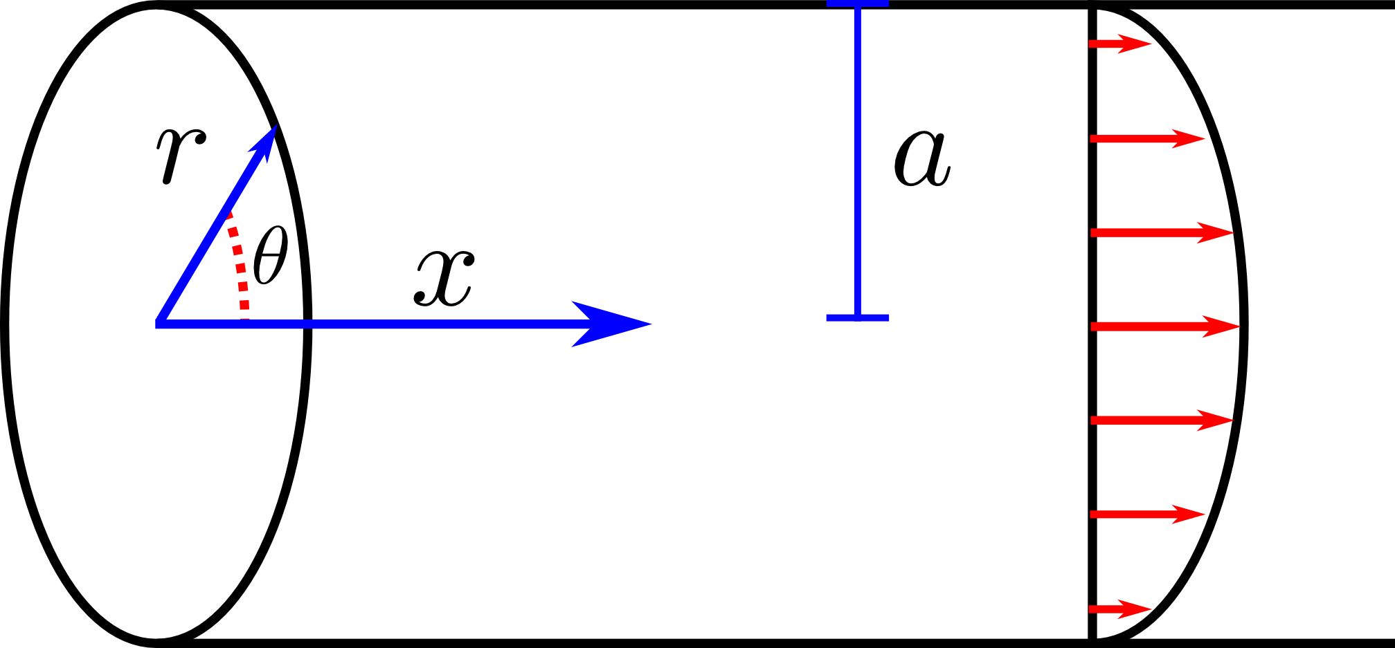
Poiseuille Flow
Let us consider the situation of steady flow through a circular tube. For this situation we’ll use a cylindrical coordinates system with  being the radial coordinate,
  being the angular coordinate and
  being the coordinate directed up along the symmetry axis of the tube.
For this situation we once again consider a steady flow, which means:
![\[\frac{\partial}{\partial t} = 0\]](https://sammorrell.co.uk/wp-content/ql-cache/quicklatex.com-bc2b6412afcd886f5d5b47a718e0f09b_l3.png "Rendered by QuickLaTeX.com")
We also assume that the problem is axially symmetric, which means that there’s no angular dependence in the problem:
![\[\frac{\partial}{\partial \theta} = 0\]](https://sammorrell.co.uk/wp-content/ql-cache/quicklatex.com-b77b80cda4fe8113e4ddeebd0d9f5ceb_l3.png "Rendered by QuickLaTeX.com")
Another simplification that we can make is that the pipe is semi-infinite, which means that the flow will remain constant along the pipe and won’t vary with :
![\[\frac{\partial \vec{u}}{\partial x} = 0\]](https://sammorrell.co.uk/wp-content/ql-cache/quicklatex.com-332078e98f5d44eb45b106e7d343c215_l3.png "Rendered by QuickLaTeX.com")
One of the important equations in fluid dynamics is the continuity equation, which enforces mass conservation on the mathematics. Put simply, as material flows in and out of our parcel of data, none of it is allowed to go missing. The continuity equation for a Newtonian fluid is ( ), but under all of these simplifications we’ve made it becomes:
![\[\frac{1}{r} \frac{\partial (r U_r)}{ \partial r} + \cancelto{0}{\frac{1}{r} \frac{\partial U_\theta}{\partial \theta}} + \cancelto{0}{\frac{1}{r} \frac{\partial U_x}{\partial x}} = 0\]](https://sammorrell.co.uk/wp-content/ql-cache/quicklatex.com-948e5ffe287ed2c81f6de8b5284c69c1_l3.png "Rendered by QuickLaTeX.com")
![\[\implies \frac{1}{r} \frac{\partial (r U_r)}{ \partial r} = 0\]](https://sammorrell.co.uk/wp-content/ql-cache/quicklatex.com-ad0b4d8f3c7c8036a220781e0dff5fd8_l3.png "Rendered by QuickLaTeX.com")
Therefore, we can reduce the -component of the Navier-Stokes equation to:
![\[0 = \underbrace{- \frac{d P}{d x}}_\text{A} + \underbrace{\frac{\mu}{r} \frac{\partial}{\partial r} \left( r \frac{\partial U_x}{\partial r} \right)}_\text{B}\]](https://sammorrell.co.uk/wp-content/ql-cache/quicklatex.com-852b677e7d9ac27c6e1212c11e28f929_l3.png "Rendered by QuickLaTeX.com")
This allows the problem to be solved analytically; as the non-linear inertial term vanishes. Much of the complexity in solving these equations comes from the inertial term. We now take a look at the component:
![\[0 =\ - \frac{\partial p}{\partial r} + \cancelto{0}{\frac{\mu}{\rho} \nabla^2 U_r}\]](https://sammorrell.co.uk/wp-content/ql-cache/quicklatex.com-74eee32ae8248a87ff4589957050e521_l3.png "Rendered by QuickLaTeX.com")
We can now see that  , which means that
  is not a function of . If we now consider parts
  and
and  of the component, we can also see that both terms in that equation must be constant along the pipe; because should only be a function of and should only be a function of . Given this fact,
  must be constant. This means that pressure must vary linearly along the pipe. We can now integrate the momentum equation along the tube to get:
![\[U = \frac{r^2 - a^2}{4 \mu} \left( \frac{d p}{d x} \right)\]](https://sammorrell.co.uk/wp-content/ql-cache/quicklatex.com-6a2603a19f2f6e5d65da944f4d58b746_l3.png "Rendered by QuickLaTeX.com")
This gives you the flow through the tube. Using this equation it’s possible to also figure out the volume flow rate and other properties. This particular problem may seem a little contrived, however it’s actually very useful. This result is valid for any fluid flowing through a pipe; given the correct conditions. This has applications for modeling prototypes in engineering. Other situations where you could apply this is modeling the ascent of magma through the lithosphere and flow of blood through vessels.
In the Context of Planets
My interest in all of this mathematics is in the context of planetary atmospheres. I’ve always been intrigued by the work of the Met Office in Exeter and their modelling of our atmosphere. It’s impressive how they can manage to model such a chaotic system and be as accurate as they are with weather forecasting. The cool thing about their work is that it doesn’t just apply to this planet. If you strip out all of the things that apply specifically to the Earth it’s an exceedingly powerful tool for modelling the atmospheres of other planets. This is just what the astrophysics group at the University of Exeter is doing. One of the papers from this research is down in the references. There’s a lot more that we can go into, so in my next post I’ll describe some of the hydrodynamics which is especially useful for dealing with planetary atmospheres. Until then thanks very much for reading.
References
- Browning, M. (2014, November). Solar and Extrasolar Planets and their Atmospheres.
- Kundu, P. K. & Cohen, I. M. (2010). Fluid Mechanics. Burlington, USA: Academic Press.
- Mayne, N. J. et al (2014). The UM, a fully–compressible, non–hydrostatic, deep atmosphere GCM, applied to hot Jupiters, ArXiv e-prints.
