In my last post I went over a really powerful bit of physics called fluid mechanics, which describes the flow of fluid through a system. The main equation in this framework is the momentum equation; the Navier-Stokes equation.This equation is nye on impossible to solve analytically in it’s full grotesque glory, so in the last post I discussed some of the useful problems we can consider that allow us to simplify and actually solve this equation. These approximations are generally very useful, but given a context we can make further specialisations to this equation which make the results even more useful. Because we’re astrophysicists wanting to study complex, chaotic systems, what better system to focus on than a planetary atmosphere. This is just what I will do in this post.
The Coriolis Term
I alluded to this briefly in the previous post, but I’ll go a little more in-depth this time. In the previous examples we made the assumption that the system we were studying was an inertial frame of reference, that is that all laws of physics hold within the frame; most importantly Newton’s first law of motion: an object at rest or moving at a constant velocity will remain doing so until acted on by an external resultant force. The problem is that this isn’t true of a rotating planet. Because of this we introduce an effect known as the Coriolis force. This is a fictitious force exerted on a body when moving in a rotating reference frame. It’s called “fictitious” as it’s not technically a force; merely the affect of measuring relative to a rotating coordinates system. Despite this complication, it can be corrected for by adding a term to the momentum equation we discussed last time, the Coriolis term. With this term added the momentum equation takes the form of:
![\[\frac{\partial \vec{v}}{\partial t} + \vec{u} \cdot \nabla \vec{u} = \ - \frac{1}{\rho} \nabla P + \vec{g} + \nu \nabla^2 \vec{v}\ - 2 \vec{\Omega} \times \vec{u}\]](https://sammorrell.co.uk/wp-content/ql-cache/quicklatex.com-34b64de1108dcc4a6012a089e9bd294b_l3.png "Rendered by QuickLaTeX.com")
where  is the rotation rate of the planet. Now that we have this important term added to the equation we can go and study some atmospheres.
Geostrophic Wind
If we consider a terrestrial planet, like Earth, the atmosphere and oceans make up a vertical layer that is small in comparison to the radius of the rest of the planet. On this occasion we’re comparing something in the order of kilometres thick to something that is hundreds or thousands of kilometres in radius. This suggests that we may indeed expect vertical velocity in the  direction to be small as a result. Now also consider that we’re considering length scales small enough that the curvature of the Earth can be ignored. This allows us to consider a system on a plane tangential to the surface of the planet.
For this next section we introduce a new quantity, the Coriolis Parameter  ; and for a planet this defined as:
![\[f = 2 \Omega \sin(\phi)\]](https://sammorrell.co.uk/wp-content/ql-cache/quicklatex.com-e1609fe59fda406518d97f578b7b431e_l3.png "Rendered by QuickLaTeX.com")
where  is the rotation rate of the planet and
  is the latitude of the point on the surface at which we are studying the tangent. Studying this parameter we can see that where latitude is
  at the equator, will vanish. However, if we
have as  , the case at the poles, this parameter is maximal and comes out as
  . This parameter causes an apparent force to act in a direction perpendicular to the direction of the fluid flow; to the right of it in the northern hemisphere and to the left in the southern hemisphere. It should be pointed out that, as the actual force is dependent on
  , the Coriolis force cannot cause wind to move, but merely change its direction.
Rossby Number
It’s at this juncture that it’s convenient to define another non-dimensional number; like the Reynolds number we discussed in the last post. If we now take the horizontal equation of motion for a fluid in the tangential reference frame we discussed in the previous section, we find that:
![\[\frac{\partial \vec{u}}{\partial t} + (v \cdot \nabla) \vec{u} + \vec{f} \times \vec{u} = \frac{1}{\rho} \nabla_z P\]](https://sammorrell.co.uk/wp-content/ql-cache/quicklatex.com-800b22414243219bc2cdcb0f128daca7_l3.png "Rendered by QuickLaTeX.com")
where  is the Coriolis term including the Coriolis parameter. If we now take
  to be a horizontal velocity scale and
  to be a horizontal length scale we find that the non-linear acceleration term and Coriolis term come out as
  and
and  respectively. We can now define the Rossby number by taking the ratio of these scaled terms:
![\[Ro \equiv \frac{U}{fL}\]](https://sammorrell.co.uk/wp-content/ql-cache/quicklatex.com-cebc88c1784eb812546897d40d06cfe8_l3.png "Rendered by QuickLaTeX.com")
This non-dimensional number characterises the importance of rotation on the fluid. If the Rossby number is small, it is suggested that the effects of rotation is important for a given fluid. Taking values typical for a large-scale flow of an atmosphere ( ) we find that this is the case.
Geostrophic Flow
If the Rossby number is small enough then the rotation term in the horizontal flow equation above will dominate over the non-linear advection term. If the time period of the motion scales with the advective term, rotation also dominates over the local acceleration
term. This leaves us with only the horizontal pressure gradient to balance the Coriolis force.
![\[\vec{f} \times \vec{u} \sim \frac{1}{\rho} \nabla_z P\]](https://sammorrell.co.uk/wp-content/ql-cache/quicklatex.com-f8e3957cb8627ec67fc2ebbcb928496a_l3.png "Rendered by QuickLaTeX.com")
This balance is called geostrophic balance, and is very useful in the context of geophysical fluid dynamics. It’s at this point that we take the determinant of the cross product matrix of to attain the two horizontal components of velocity in our tangential plane:
![\[-\ f u \equiv \frac{1}{\rho}\frac{\partial P}{\partial y} \quad \text{and} \quad f v \equiv -\ \frac{1}{\rho} \frac{\partial P}{\partial x}\]](https://sammorrell.co.uk/wp-content/ql-cache/quicklatex.com-1b30a03f6750eb664f67c16bfe3283be_l3.png "Rendered by QuickLaTeX.com")
In the direction, we simply have hydrostatic equilibrium, which, if you recall, is where the pressure gradient is in direct balance with gravitational acceleration:
![\[\frac{\partial P}{\partial z} = - \rho g\]](https://sammorrell.co.uk/wp-content/ql-cache/quicklatex.com-8aaa0705918009030520d6731aed403f_l3.png "Rendered by QuickLaTeX.com")
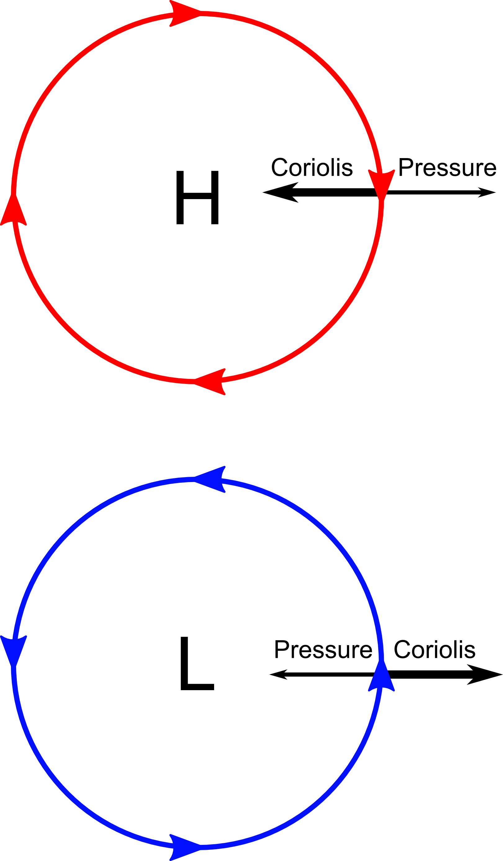
There are a number of consequences of this approximation. The most important is geostrophic flow. This implies through the mathematics that, since the two dominant effects in a rotating planetary system are rotation and pressure gradients and that they are both balancing one another, the flow of the atmosphere will tend to follow lines of constant pressure, or isobars. The direction of this flow depends on the Coriolis parameter and the pressure gradient in question. If  , such as in the northern
hemisphere of the Earth, the flow will be anti-clockwise around a region of low pressure (cyclonic flow) and clockwise around a region of high pressure (anticyclonic flow). In the southern hemisphere, where  , the inverse of this is true.
The Taylor-Proudman Effect
An important result of geostrophic balance in a homogeneous fluid is the Taylor-Proudman Effect. This effect isn’t generally observed in the atmosphere, but it’s a
remarkable piece of fluid mechanics none the less. If we consider a piece of the atmosphere as if it were at one of the poles, we can lose the cosine in the Coriolis parameter and our equations of geostrophic balance will reduce to:
![\[ - 2 \Omega v = - \frac{1}{\rho} \frac{\partial P}{\partial x}\]](https://sammorrell.co.uk/wp-content/ql-cache/quicklatex.com-0a946ab76c3cfbc96655af24b3eab25f_l3.png "Rendered by QuickLaTeX.com")
![\[ 2 \Omega u = - \frac{1}{\rho} \frac{\partial P}{\partial y}\]](https://sammorrell.co.uk/wp-content/ql-cache/quicklatex.com-28d5f31eae3ffdfd81dd09e1cfb66595_l3.png "Rendered by QuickLaTeX.com")
![\[0 = - \frac{1}{\rho} \frac{\partial P}{\partial z} - g\]](https://sammorrell.co.uk/wp-content/ql-cache/quicklatex.com-597ae03c3b82f87a4c21a62f657750d7_l3.png "Rendered by QuickLaTeX.com")
It’s useful now to define one more non-dimensional number, the Ekman number. The Ekman number is the ratio of the viscous term and the Coriolis term. If we adopt the same length scale analysis as we did previously, we end up with this:
![\[\text{Ekman number} = \frac{\text{viscous term}}{\text{Coriolis term}} = \frac{\rho v U / L^2}{\rho f U} = \frac{v}{f L^2} = E\]](https://sammorrell.co.uk/wp-content/ql-cache/quicklatex.com-6627dc45c39776969cf2128b95167a47_l3.png "Rendered by QuickLaTeX.com")
In the regime we are considering both the Rossby number  and the Ekman number
  are small; meaning that the Coriolis term is dominating. By cross differentiation between the equations above we can find that:
![\[2 \Omega \left( \frac{\partial v}{\partial y} + \frac{\partial u}{\partial x}\right) = 0\]](https://sammorrell.co.uk/wp-content/ql-cache/quicklatex.com-03943d885bb81410f43422038dcb165e_l3.png "Rendered by QuickLaTeX.com")
Using the continuity equation, defined as  , we can also show that
  . Differentiating the equations of geostrophic balance with respect to
  also gives:
![\[\frac{\partial u}{\partial z} = \frac{\partial v}{\partial z} = 0\]](https://sammorrell.co.uk/wp-content/ql-cache/quicklatex.com-5e7381fdd6132f4f7e2d48c7a98b583a_l3.png "Rendered by QuickLaTeX.com")
This leads us to the conclusion that
![\[\frac{\partial \vec{u}}{\partial z} = 0\]](https://sammorrell.co.uk/wp-content/ql-cache/quicklatex.com-1f82c59af2e10da3e534f36192e46047_l3.png "Rendered by QuickLaTeX.com")
This means that the motion of the fluid cannot vary in the direction of the rotation axis . This leads to the interesting phenomena that for a barotropic, rotating fluid, motion must be constant along cylinders parallel to the rotation axis.
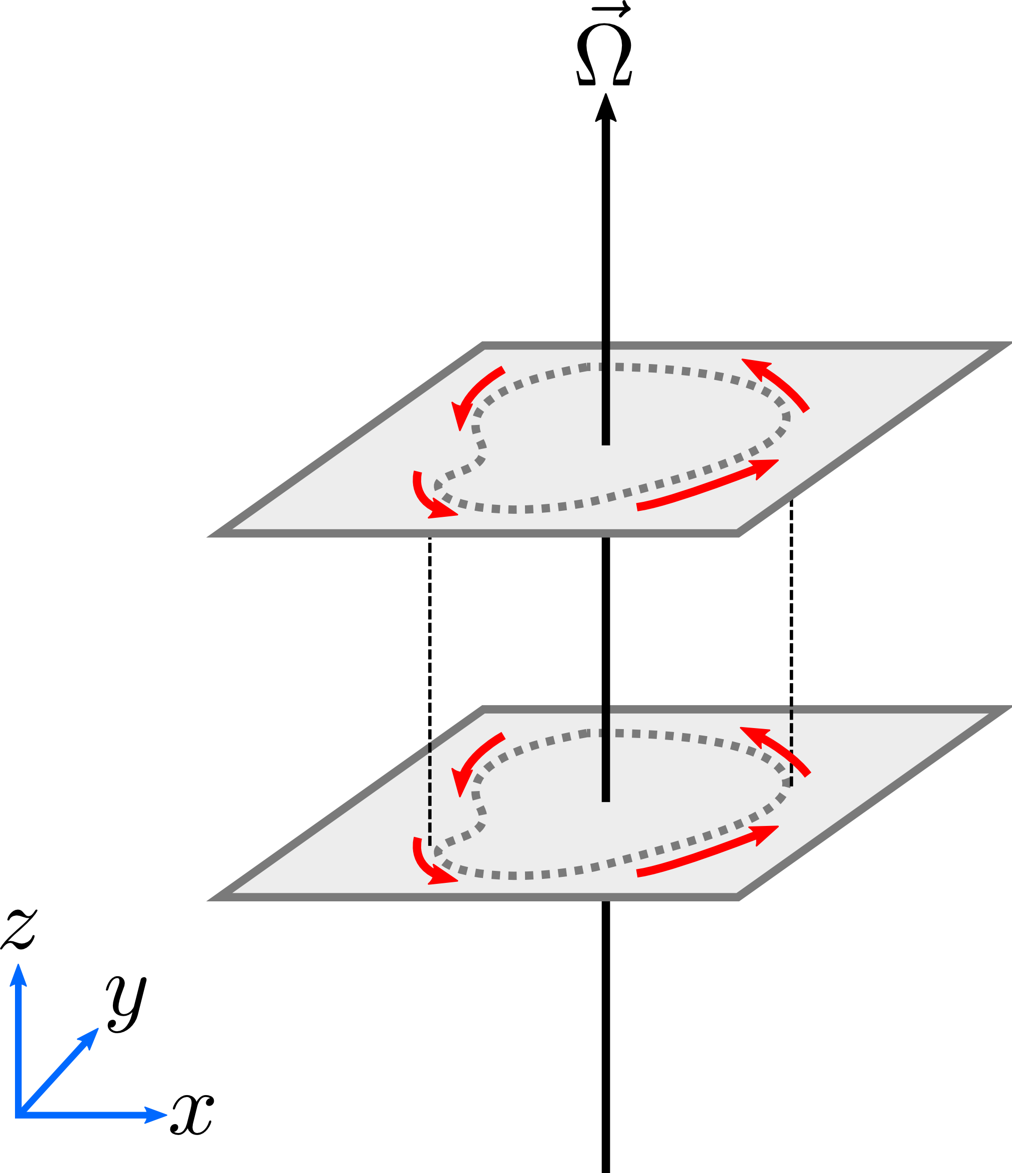
This image shows the Taylor-Proudman effect in action. What is illustrated is two layers of atmosphere orientated in the  plane, orthogonal to the rotation axis of the planet . As dictated by the Taylor-Proudman theorem, the motion of the fluid is constant along the rotation axis.
Thermal Wind Balance
Using the equations of geostrophic balance and hydrostatic equilibrium, it’s possible to show that, due to a horizontal gradient of density, the wind develops a vertical shear. We can do this by eliminating  from the equations we attain by considering geostrophic balance in the horizontal plane, like so:
![\[\frac{\partial v}{\partial z} =\ - \frac{g}{\rho_0 f} \frac{\partial \rho}{\partial x}\]](https://sammorrell.co.uk/wp-content/ql-cache/quicklatex.com-507c59af58ba5ceb3ec6d90424612061_l3.png "Rendered by QuickLaTeX.com")
![\[\frac{\partial u}{\partial z} = \frac{g}{\rho_0 f} \frac{\partial \rho}{\partial y}\]](https://sammorrell.co.uk/wp-content/ql-cache/quicklatex.com-80e9c6d8566c333e9c8cceeeac1f3a33_l3.png "Rendered by QuickLaTeX.com")
where  is the average density of the fluid. These are called the thermal wind equations, because they give the vertical variation of wind from horizontal temperature gradients. Thermal wind is baroclinic, meaning that its density depends on both density and pressure, because the surfaces of constant and
  never coincide. Let’s just suppose that we have a horizontal gradient of density such that the contours of constant density slope downward with increasing
  .
.

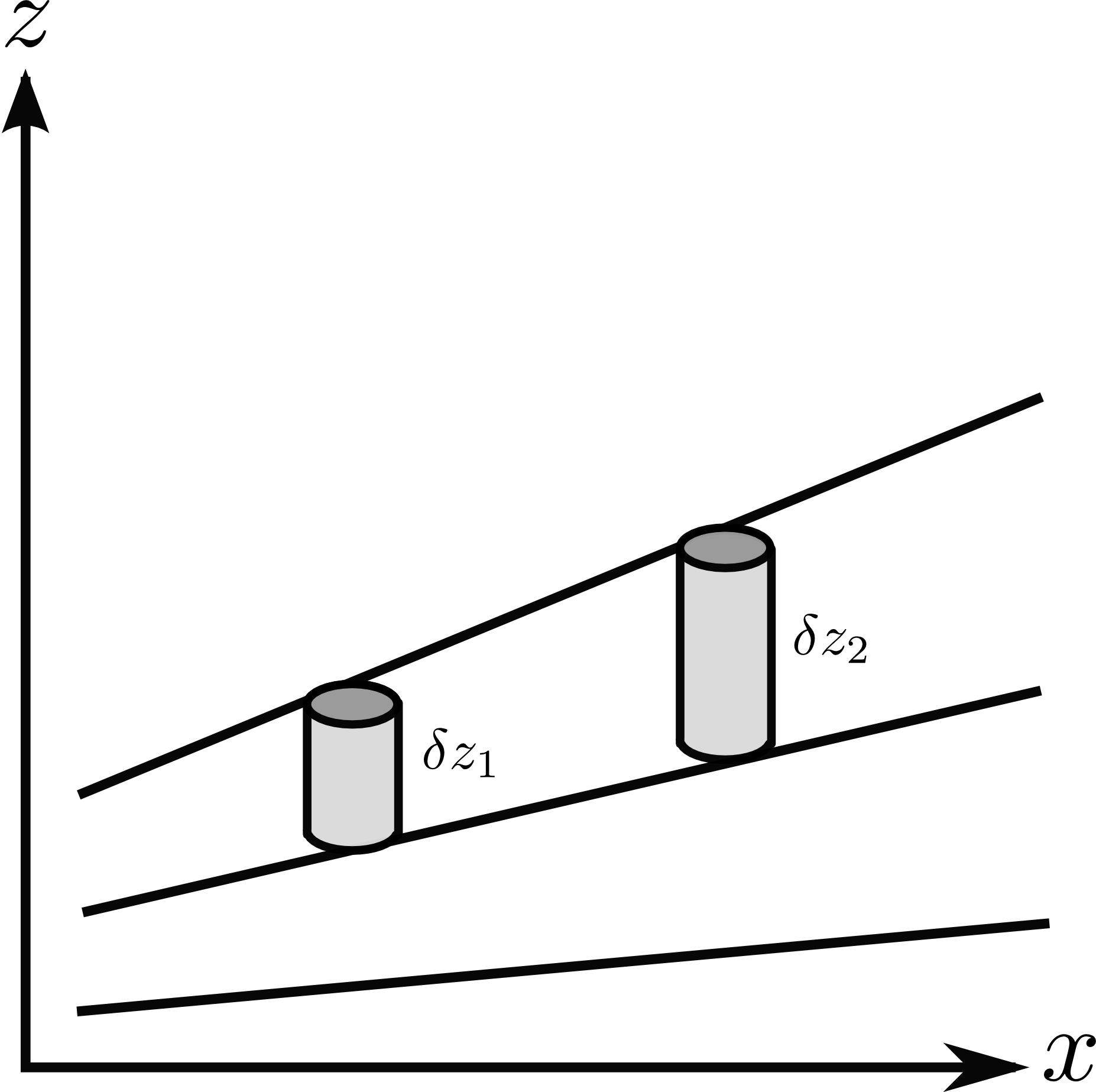
In this plot:
![\[\rho_0 > \rho_1 > \rho_2\]](https://sammorrell.co.uk/wp-content/ql-cache/quicklatex.com-dceed795bedde990afc85fe57ca1bed6_l3.png "Rendered by QuickLaTeX.com")
Due to the hydrostatic equilibrium constraint we imposed on vertical momentum earlier, there will be a positive  which increases with height. We take two columns of the material
  and
and  between two isobars whose
weights are required to be equal. Due to density increasing with decreasing , in the situation of a baroclinic atmosphere, the separation between isobars must increase with increasing . As density is decreasing as a function of , the volume of atmosphere between the isobars is required to increase to satisfy the constraint that the weights of and must be equal.
If the fluid is in geostrophic balance the pressure gradient that is
created here will be balanced by Coriolis forces; a velocity in the
 direction which increases with height.
The Boussinesq Approximation
Generally speaking, density perturbations in the atmosphere are quite small when compared to the mean density. Thus, it was suggested in 1903 by Joseph Valentin Boussinesq that density perturbations in a fluid can be completely neglected unless they are due to gravity; terms where is multiplied by acceleration due to gravity  . The approximation relies on the fluid being incompressible; meaning that the equation of continuity for the fluid is simply
  . In the regime of the Boussinesq approximation compressibility effects are small, so all perturbations in density come from temperature changes. As we are considering small perturbations in a largely homogeneous, incompressible medium, it’s convenient to consider a fluid with uniform mean density and pressure
  and consider small perturbations of the fluid, such that total density and pressure are
  and
and  respectively. This approximation applies only to low Mach number flow, as the compressibility effects of the fluid are large at large Mach numbers, generating large pressure changes which cause large density changes. It’s also assumed that properties of the fluid, such as it’s stress viscosity
  , thermal diffusivity
  and specific heat capacity
  remain constant. All of these considerations to rewrite the Navier-Stokes equation as:
![\[(\rho_0 + \delta \rho) \left( \frac{D \vec{u}}{D t} + 2 \vec{\Omega} \times \vec{U} \right) =\ - \nabla \delta \rho\ - \frac{\partial P_0}{\partial z} \hat{z}\ - g(\rho_0 + \delta \rho) \hat{z}\]](https://sammorrell.co.uk/wp-content/ql-cache/quicklatex.com-18591fec8b3504dbffe3d94f1c236942_l3.png "Rendered by QuickLaTeX.com")
If we assume hydrostatic equilibrium, that  , then this can be simplified to:
![\[ (\rho_0 + \delta \rho) \left( \frac{D \vec{u}}{D t} + 2 \vec{\Omega} \times \vec{U} \right) =\ - \nabla \delta\rho\ - g \delta \rho \hat{z}\]](https://sammorrell.co.uk/wp-content/ql-cache/quicklatex.com-c2bfc1701cf968447f69ecd2e7271a9d_l3.png "Rendered by QuickLaTeX.com")
If density variations  are adequately small, then this becomes:
![\[\frac{D \vec{u}}{D t} + 2 \vec{\Omega} \times \vec{u} =\ - \nabla \phi + b \hat{z}\]](https://sammorrell.co.uk/wp-content/ql-cache/quicklatex.com-518d655187471b7fb26b1479f338406b_l3.png "Rendered by QuickLaTeX.com")
which is the equation of momentum in the Boussinesq approximation. In this equation  is the buoyancy term and
  .
.
From this it’s easy to see that hot fluids tend to rise and that cool fluids tend to sink, due to buoyancy. Given that density and temperature  are related by the equation:
![\[\rho = \rho_0 \left[ 1 - \alpha \left( T - T_0 \right) \right]\]](https://sammorrell.co.uk/wp-content/ql-cache/quicklatex.com-000265b1f4b5946b041f8ea87246abf0_l3.png "Rendered by QuickLaTeX.com")
where, as with density and pressure,  is the mean temperature of the fluid and is the total temperature and
  is the thermal expansion coefficient for the fluid.
The final outcome of both this approximation and the thermal wind balance suggest primitive versions of the Hadley Cell. This a structure in the atmosphere in which warm, moist air rises into the atmosphere near the equator, flows either north or south, depending on the hemisphere, and then cools and descends; returning to lower latitudes through a weaker return flow. This structure is fundamental to both our weather and climate on a global scale.
See it in Action
If you ever want to see this stuff in action in the Earth’s actual weather, there’s an amazing visualisation of NOAA’s Global Forecast System (GFS) data on a 3D globe. In this particular visualisation you can see many different data overlays, such as wind speed, humidity and even total cloud water to name a few. You’ll almost immediately notice how the theory of geostrophic balance affects the global flow of the winds; as you’ll be able to tell which pockets of vorticity are high or low pressure in their respective hemispheres. This in turn can tell you many things about the weather in a given location and is indeed one of the main mechanism meteorologist used to give accurate weather forecasts.
The map is available at http://earth.nullschool.net/ and I highly recommend going to watch it. It’s mesmerising. I hope I have helped a little with the complex subject of fluid mechanics and if you have been, thanks for reading.
References
- Browning, M. (2014, November) Solar and Extrasolar Planets and their Atmospheres.
- Vallis, G. K. 2006. Atmospheric and Oceanic Fluid Dynamics:
Fundamentals and Large-Scale Circulation. Cambridge University Press.
745 pp. http://www.vallisbook.org - Kundu, P. K. & Cohen, I. M. (2010). Fluid Mechanics. Burlington, USA: Academic Press.
