A little while ago I got carried away on a little post which discussed a really cool little bit of physics called radiative transfer. As I said then, radiative transfer is a technique that you can use to study how energy, in the form of electromagnetic radiation, moves through material. In that post, which you can find right here, I discussed some of the mathematics behind the technique as well as a derivation of the equation of radiative transfer. However, in that post I was a little light on actual practical applications. One use of radiative transfer is to model the effect that dust has on light as it passes through it; a phenomena known in astrophysics as extinction. This is what my current masters research entails and the models built into the code I use contain direct results of radiative transfer. However, this is most definitely not it’s only use. One rapidly expanding field of research is exoplanetary atmospheres, and radiative transfer is also extensively used for this. In this post I’ll give you a bit of insight into how exoplanet atmospheres are studied using radiative transfer and some of the important pieces of physics that can be releaved.
A Brief Reminder of Radiative Transfer
If you’ll recall, in my previous post on radiative transfer we considered a slab of material with an absorption coefficient  and emission coefficient
  . These coefficients tell us how the material absorbs and emits electromagnetic radiation. We can use the absorption coefficient to tell us how opaque or transparent a material is. We call this measure the optical depth
  , and for a slab of homogeneous material it’s given by:
![\[\tau_{\nu} = \alpha_\nu s\]](https://sammorrell.co.uk/wp-content/ql-cache/quicklatex.com-e883802ee7a4631f6ab80bdd97634523_l3.png "Rendered by QuickLaTeX.com")
where  is the length of the path that the radiation is travelling through the material. A key point to remember in the rest of this post is that an observer capturing light travelling through this material can see roughly to where
  . The specific intensity
  along a line, the intensity of light at one specific frequency
  , is governed by a differential equation:
![\[\frac{d I_\nu}{d s} = j_\nu - \alpha_\nu I_\nu\]](https://sammorrell.co.uk/wp-content/ql-cache/quicklatex.com-3fdafbb5bebefe3a93d4351b6727e33e_l3.png "Rendered by QuickLaTeX.com")
which gives the formal solution
![\[I_\nu (\tau_\nu) = I_\nu (0) e^{- \tau_\nu} + \int^{\tau_\nu}_0 S_\nu (\tau^{\prime}_\nu) e^{- (\tau_\nu - \tau^{\prime}_\nu)} d \tau^{\prime}_\nu\]](https://sammorrell.co.uk/wp-content/ql-cache/quicklatex.com-8079be59e195ac2305edb9f397b50255_l3.png "Rendered by QuickLaTeX.com")
where  is the source function, defined as
![\[S_\nu = \frac{j_\nu}{\alpha_\nu}\]](https://sammorrell.co.uk/wp-content/ql-cache/quicklatex.com-cb65218571eb47f34a197d4c80f03ddf_l3.png "Rendered by QuickLaTeX.com")
Now that we have these pieces of mathematics in place, we can do some interesting things with atmospheres.
What’s it Made From?
One important result of radiative transfer is that the intensity is specific to a certain wavelength of light, so just by observing the systems we’re studying at a different wavelength we can see different results. For example the Atmosphere of the Earth is fairly transparent to visible light, however due to all of the water and carbon dioxide in our atmosphere, it’s fairly opaque at most infrared wavelengths. Thanks to this knowledge, physicists can study the composition of atmospheres light years away from us. I’ll describe how this works in a minute, but first a little on exoplanet detection.
This shows a schematic view of the transit method for detecting exoplanets. The planet passes in front of the star and blocks out a small part of the light. The light curve underneath shows roughly what you’d see if you plot the flux from the star over time.
Most exoplanets are detected now using a technique called the transit method, where the planet moves in between the observer and the star it’s orbiting, blocking out some of the light. This method can yield many properties of the planet, such as it’s size, distance from the star and orbital period. With planets that have an adequately thick atmosphere, we can also determine what the atmosphere is made of. This works because different chemical components of the atmosphere interact with light in a different way.
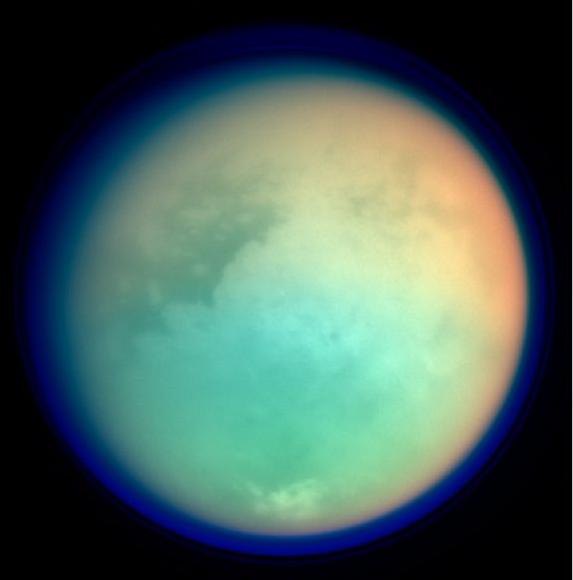
This is a false colour image of Saturn’s moon, Titan. It’s assembled from 4 images from the Casinni probe. The colours in the image represent infrared (red and green) and ultraviolet (blue). This elegantly demonstrated how some wavelengths are more opaque than others and how this changes due to atmospheric composition. The red and green colours show areas where methane in the atmosphere is absorbing IR radiation and the blue shows the height of the atmosphere and detached hazes. Image Credit: NASA/JPL/Space Science Institute.
The image of Titan above shows how the atmosphere can appear different heights when observed at different different wavelengths. If this were a planet, measuring the flux in the infrared (green and red in the image) would make it appear smaller than if it were measured in the UV (blue). This is a similar principle to how transit spectrophotometry works. By measuring the dip in the light curve as the planet transits in front of its star, a picture can be built up of how the atmosphere responds to different wavelengths of light. This is one of the main methods used to study the atmospheric composition of planets around other stars.
Mathematically, what determines an atmosphere’s appearance is the optical depth  and the source function
  of the atmosphere. If we consider the formal solution of the equation of radiative transfer that I showed you earlier in this post, we can take it apart and see what’s happening. We take the light from the star to be
  and if there is nothing in the way, it will reach us at the same intensity. However, if we place the atmosphere of a planet in the way it starts to attenuate this light; hence the
  factor in the same term, which causes an exponential fall off with increasing optical depth. The second term is responsible for modelling absorption and emission from the atmosphere. The integral is used to sample the material along the path that will be visible to us, attenuating the intensity as dictated by the source function.
The Greenhouse Effect
A practical consequence of this mathematics is the commonly misunderstood greenhouse effect. This process is caused by chemical species in the atmosphere, such as carbon dioxide, absorbing infrared radiation that is given off by the ground when heated by the Sun. If there were no greenhouse effect the equilibrium temperature of the atmosphere would be determined purely by the flux of the planet’s star on the surface. The power input is given entirely by this flux:
![\[P_\text{in} = I_0 (1 - a) \pi R_p^2\]](https://sammorrell.co.uk/wp-content/ql-cache/quicklatex.com-f95dd53511359132d1c4885dd2b0a2db_l3.png "Rendered by QuickLaTeX.com")
where  is the albedo, essentially the fraction of light that is reflected off of the surface instead of being absorbed, and
  is the radius of the planet. Now we consider the power output of the radiated planet:
![\[R_\text{out} = \epsilon \sigma A T^4\]](https://sammorrell.co.uk/wp-content/ql-cache/quicklatex.com-21e886bc8ce5e2c2a5a704656bab05c5_l3.png "Rendered by QuickLaTeX.com")
where  is the emissivity of the planet,
  is the Stefan-Boltzmann constant,
  is the temperature and
  . We can now calculate the equilibrium temperature by setting
  and stating that the planet is emitting uniformally across its surface as a blackbody, so
  . From this the equilibrium temperature of the planet is:
![\[T_\text{eq}^4 = \frac{I_0 (1 - a)}{4 \sigma}\]](https://sammorrell.co.uk/wp-content/ql-cache/quicklatex.com-426d588fc63342c1e2523ebce36257ae_l3.png "Rendered by QuickLaTeX.com")
If we consider the Earth system using this equation we find that the equilibrium temperature of the planet is  . This is obviously a pretty poor approximation of the Earth’s true
  . For a planet with a thick atmosphere, such as Venus, this merely approximates the temperature at the top of the clouds, as the clouds are opaque to long wavelength radiation. However, we can improve our approximation. If we assume that the atmosphere is in radiative equilibrium, that it’s a steady state system with an equal amount of incoming and outgoing radiative heat, and we also use the 2-stream approximation, that light in an atmosphere only travels in two discrete directions, we can work out the surface temperature of the planet. From these two considerations we can get the flux:
![\[F(z) = - \frac{16}{3 \rho} \frac{\partial T}{\partial z} \frac{\sigma T^3}{\kappa}\]](https://sammorrell.co.uk/wp-content/ql-cache/quicklatex.com-7c1ae88c220b01ca3220a669f60830f8_l3.png "Rendered by QuickLaTeX.com")
Where  is the density of the atmosphere and
  is the absorption coefficient. From this it follows that:
![\[T^4(\tau) = T_0^4 \left( 1 + \frac{3}{2} \tau \right) \quad \text{where} \quad T_0^4 = \frac{1}{2} T_\text{eq}^2\]](https://sammorrell.co.uk/wp-content/ql-cache/quicklatex.com-3fc60f9e6a71fddc5db6ee31bdb5eccd_l3.png "Rendered by QuickLaTeX.com")
Then using this we can derive the surface temperature:
![\[T_s^4 = T_\text{eq}^4 \left( 1 + \frac{3}{4} \tau_s \right)\]](https://sammorrell.co.uk/wp-content/ql-cache/quicklatex.com-30dce4af37ce610cbfe7b74eadad536f_l3.png "Rendered by QuickLaTeX.com")
This is a very important relation in atmospheric science, especially in astrophysics, as it allows you to relate together temperature and optical depth  in an atmosphere; as such it’s commonly labelled the
  relation.
Active Research
The astrophysics group at the University of Exeter are currently doing a lot of research on exoplanet atmospheres; which includes studying the atmospheric composition as well as the climates of exoplanets, which I will go into in another post. The atmospheric compositions of hot Jupiters is an especially active field of research. Hot Jupiters are Jupiter-like exoplanets that are exceedingly close in to their parent star, most far closer than Mercury is to our Sun. Hannah Wakeford and Dr. David Sing have recently released a paper which details cutting edge results in this field. Using a process called transmission spectroscopy, where you study the light that gets transmitted through the atmosphere of the exoplanet, you can clearly see chemical condensates that could form clouds. So, not only can we now detect exoplanets and work out some intrinsic and important properties of them, but we’re now on the edge of actually studying their atmospheric composition and even now their climate, all thanks to the physics of radiative transfer.
I hope you’ve enjoyed this post. I enjoy writing this stuff, but it takes time because I like to try and make sure that I have all of my mathematics correct and my facts straight. If you notice something incorrect, please don’t hesitate to let me know, then I’ll correct it and give credit where it’s due. I’m cooking up a few posts on some basic fluid mechanics but until then, thanks for reading.
References
- Browning, M. (2014, November). Solar and Extrasolar Planets and their Atmospheres.
- Nimmo, F. (2011) EART164: Planetary Atmospheres (Week 10 – Recap)
- Rutten (2003) Radiative Transfer in Stellar Atmospheres
- Wakeford, H. R.; Sing, D. K. (2014) Transmission spectral properties of clouds for hot Jupiter exoplanets
