It’s deep in exam season for me at the moment, which means that if you try talking to me, chances are that I’ll have my head in a book. I talked a while back about solving radiative transfer problems with Monte Carlo methods, but I never actually went very far into how radiative transfer works. Without further adieu, here’s a brief intro to radiative transfer. I’m going to assume a little basic knowledge of algebra and calculus, but not too much.
What is Radiative Transfer?
Radiative transfer describes how electromagnetic waves, such as light, interact with a material as it travels through it. At the core of this topic is a very powerful equation, called the equation of radiative transfer. Using this equation, we can find solutions for a ton of different problems in Astrophysics, I’ll go through some applications a little later on. Let’s set up our problem.
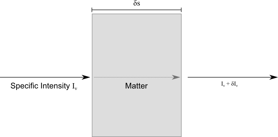
The diagram above details one of the simplest problems we can tackle in radiative transfer. Let’s consider a block of some material which is the same all the way through (homogeneous). We have some radiation coming in from the left, passing straight through and interacting with the material in this block and coming out and continuing on its path on the right. The job of radiative transfer is to describe how the light interacts with the material. To do this we consider the intensity of the incident radiation, measured in energy per unit surface area, at a specific frequency between  and
and  . This is called the specific intensity and is given the symbol
  . To proceed any further, we need to consider how the material interacts with the radiation.
Dealing with the Material
Light interacts with the electromagnetic fields within the material. For a complete description of the system, we’d need to go down into quantum mechanics and relativistic electromagnetism. However, since we’re dealing with many, many photons and radiative transfer is purely a macroscopic description of the system, we can simplify how we deal with these interactions by introducing the absorption coefficient  and the emission coefficient
  .
.
The absorption coefficient acts to reduce the total specific intensity of the system. This is due photons being absorbed by atoms and molecules in the material. The emission coefficient acts to increase the specific intensity by accounting for the light the material emits. This is often due to atoms that were excited by photon absorption re-emitting those absorbed photons. There is generally another phenomena involved in radiative transfer, called scattering. This is when the energy from photons isn’t removed from the radiation as is the case in absorption, but is simply diverted from its straight trajectory through a solid angle  due to ‘bouncing’ off of a molecule or atom. Since the system we are considering here is effectively one-dimensional, as well as making the maths a lot easier, we’re going to ignore scattering. In our solution, we’re going to be using the ratio of these two quantities, called the Source Function, defined by:
![\[\Sigma_{\nu} \equiv \frac{j_{\nu}}{\alpha_{\nu}}\]](https://sammorrell.co.uk/wp-content/ql-cache/quicklatex.com-1686c6f0026585cb5e3a93c652a88261_l3.png "Rendered by QuickLaTeX.com")
This quantity is the measure of how photons are added and removed from the radiation due to the material its passing through. This will be an important part of our solution.
Optical Depth
Optical depth  is a measure of how transparent the block of material is. It tells you the how much of the incident radiation
  that is neither scattered or absorbed while travelling through the material, and comes out as
  . It is defined as:
![\[\frac{I_{\nu} + \delta I_{\nu}}{I_{\nu}} = e^{- \tau_{\nu}}\]](https://sammorrell.co.uk/wp-content/ql-cache/quicklatex.com-bf8c95754b294a3c696d267188b93653_l3.png "Rendered by QuickLaTeX.com")
The optical depth is actually related to the absorption coefficient. In this simple example the only thing taking away from the specific intensity is absorption. Because of this, we can simply add up the contributions of all the way along a given path in intervals of  . Therefore, we can define optical length of
  as:
as:
![\[\tau_{\nu} = \int^s_0 \alpha_{\nu}(s') ds'\]](https://sammorrell.co.uk/wp-content/ql-cache/quicklatex.com-2769f33cb7c2f093fd9508cb4e549ce3_l3.png "Rendered by QuickLaTeX.com")
Since we’re dealing with a homogeneous block of material, is constant and we can substitute the integral for a simple multiplication.
![\[\tau_{\nu} = \alpha_{\nu} s\]](https://sammorrell.co.uk/wp-content/ql-cache/quicklatex.com-c34976a8e88d7c4b1d29711031cb9f97_l3.png "Rendered by QuickLaTeX.com")
The optical depth is a particularly useful property of the block. When  the material is said to optically thick, or opaque. This means that the typical photon cannot traverse the entire block without being absorbed. Conversely, when
  the material is said to be optically thin, or transparent; meaning that the typical photon can traverse the entire block without being absorbed.
The Formal Solution to the Equation of Radiative Transfer
Now we have these building blocks in place, we can put it all together. The equation of radiative transfer is a simple, first order differential equation:
![\[\frac{\delta I_{\nu}}{\delta s}= - \alpha_{\nu} I_{\nu} + j_{\nu}\]](https://sammorrell.co.uk/wp-content/ql-cache/quicklatex.com-4ecc2df1da8674d3e802907cdaee8c64_l3.png "Rendered by QuickLaTeX.com")
To summarise, the change in specific intensity is proportional to the intensity being added by emission from the material and inversely proportional to the absorption by the material  , which itself is dependent on intensity of the radiation passing through the material
  .
.
![\[I_{\nu} = I_0 e^{- \tau_{\nu}} + \int^{\tau_{\nu}}_0 \frac{j_{\nu}}{\alpha_{\nu}} e^{- \left( \tau_{\nu} - \tau'_{\nu} \right)} d\tau'\]](https://sammorrell.co.uk/wp-content/ql-cache/quicklatex.com-8f65bab6580f63b8754591eae541a9db_l3.png "Rendered by QuickLaTeX.com")
[wpspoiler name=”Derivation of the formal solution to the Radiative Transfer Equation”]
- We start off with the equation for radiative transfer as shown above and we switch variables for optical depth . This leaves us with:
![\[\frac{d I_{\nu}}{d \tau_{\nu}} + I_{\nu} = \frac{j_{\nu}}{\alpha_{\nu}}\]](https://sammorrell.co.uk/wp-content/ql-cache/quicklatex.com-86c81c558d7498f0d2d685cd242855f8_l3.png "Rendered by QuickLaTeX.com")
You’ll now notice that we have a a term which is our source function I mentioned earlier.
- Now multiply by

![\[\frac{d(e^{\tau_{\nu}} I_{\nu})}{d \tau_{\nu}} = I_{\nu} + \frac{d I_{\nu}}{d \tau_{\nu}}\]](https://sammorrell.co.uk/wp-content/ql-cache/quicklatex.com-db87471cb59893387d9b161c12010e0f_l3.png "Rendered by QuickLaTeX.com")
![\[\frac{d(e^{\tau_{\nu}} I_{\nu})}{d \tau_{\nu}} = \frac{j_{\nu}}{\alpha_{\nu}} e^{\tau_{\nu}}\]](https://sammorrell.co.uk/wp-content/ql-cache/quicklatex.com-751d87df1aca9e8ff2a2286beeb684af_l3.png "Rendered by QuickLaTeX.com")
- We now integrate…
![\[[e^{\tau'_{\nu}} I_{\nu}]^{\tau}_0 = \int^{\tau_{\nu}}_0 \frac{j_{\nu}}{\alpha_{\nu}} e^{\tau'_{\nu}} d \tau'\]](https://sammorrell.co.uk/wp-content/ql-cache/quicklatex.com-22fccecc4e5021c768077aaf5becfd6c_l3.png "Rendered by QuickLaTeX.com")
![\[e^{\tau'_{\nu}} I_{\nu} + I_0= \int^{\tau_{\nu}}_0 \frac{j_{\nu}}{\alpha_{\nu}} e^{\tau'_{\nu}} d \tau'\]](https://sammorrell.co.uk/wp-content/ql-cache/quicklatex.com-4b21f207384f4785f0574f9a0625493a_l3.png "Rendered by QuickLaTeX.com")
You’ll note here that
 is the background intensity of the radiation.
 - We now multiply through by
 .
.
[/wpspoiler]
Limitations
This solution, despite its usefulness, has many limitations to it. As I detailed in the post, this is a simple one-dimensional mathematical description of a system. It completely ignores the phenomena of scattering. If we wish to extend this theory to more realistic situations, such as that used in numerical simulations, we need to extend the theory to three-dimensions and work scattering into equations. If we do this, we not only have to account for light entering the material at along our line of sight, but we also need to consider photons that could be scattered into our line of sight. You can see the mathematics immediately become a lot more complex.
Another limitation of radiative transfer in general is that in each calculation we can only consider a specific frequency, between  . This is principally due to the fact that absorption is heavily dependent on frequency. Atoms and molecules can only absorb photons whose energies correspond to the transitions to their excited states. Just the same, emitted photons correspond to a jump down from excited states. As well as being the reason that most variables are subscripted with , it means that if we want to consider a wide range of frequencies, we have to perform the calculations multiple times; once for each frequency. These limitations don’t devalue the solution we’ve managed to get, we just have to be aware of them should we want to apply the theory.
I hope this post has been useful to anyone and until next post, thanks for reading. 🙂
