Hey all! In my recent work I’ve been using numerical simulations involving radiative transfer, which basically means transferring energy via radiation such as light; in the form of photon packets. The way these simulations are run is via a method known quite widely in the physics world called ‘Monte Carlo Methods’. It took me a little while to get my head around how this all worked so I figured it might be worth writing a post here to try and help explain to anyone who might be in the same state I was in.
The Basics of Monte Carlo
So, what the hell is the Monte Carlo method? It’s a way of solving complex mathematical problems that are often impractical to solve analytically by taking a random sample of data, passing it through a probability distribution function, performing a deterministic computation on the output of this and then repeat. The idea here is that the law of large numbers will kick in and, after enough repetitions of this method, will yield a set of results that will close in (or converge) on the true solution of the problem. Given the repetetive nature of Monte Carlo algorithms, this methodology is often used in computational physics as a way to simulate complex systems in a relatively computationally efficient way.
It sounds complicated, but there are some really simple methods that will demonstrate how this method can be used to solve real problems. Here are two such examples.
Example: A Lorentzian
The first demo is of approximating the Cauchy-Lorentz distribution (or Lorentzian) using the Monte Carlo method. For this we need both the Probability distribution function (PDF) which is of the form…
![\[ f(x) = \frac{1}{\pi \gamma [1 + ( \frac{x - x_0}{\gamma} )^2]}\]](https://sammorrell.co.uk/wp-content/ql-cache/quicklatex.com-2eb58594a1a52b612889094db085bc7d_l3.png "Rendered by QuickLaTeX.com")
and we also need the cumulative distribution function (CDF) which is of the form…
![\[ F(x) = \frac{1}{\pi} \arctan (\frac{x - x_0}{\gamma}) + \frac{1}{2} \]](https://sammorrell.co.uk/wp-content/ql-cache/quicklatex.com-6c4dcdd427fba4076b00f2754ffe0731_l3.png "Rendered by QuickLaTeX.com")
In both of these equations  and
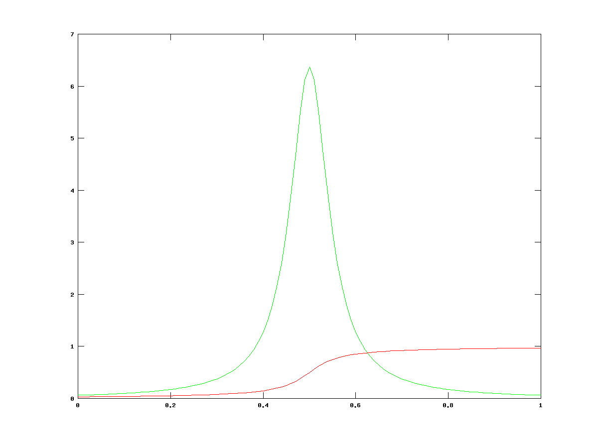
and are a scaling factor and centre of the distribution respectively. The functions that are generated by these functions are shown below on the left. the PDF is in green and the CDF is in red.
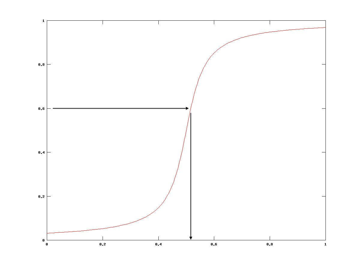
Now let’s apply Monte Carlo to randomly sample the probability distribution function. It’s this simple. Since the CDF is only defined between 0 and 1 (see for yourself in the images of the graphs) we can take our random number generator and fire numbers at an inversion of this function, which means that we’re making  the subject and we’re putting in values for
  . A demonstration of this is shown above the right. We are taking our random numbers and substituting them into the inversion. This maps them back to a value on the x-axis. From this we can add up all the x-axis hits we get and approximate the function.
If we put in a hundred random values into this and group them together into bins we get something that looks like this…
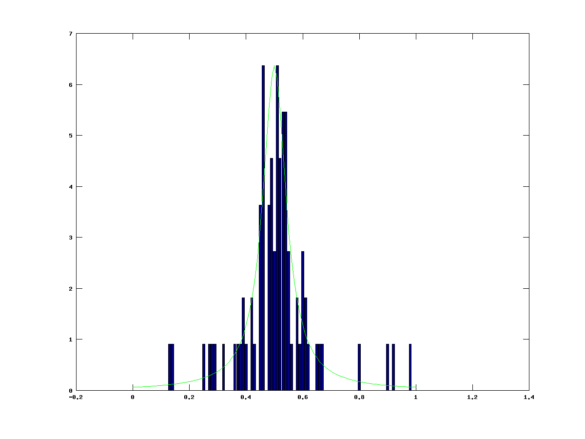
The example here shows a very rough approximation. Even with such a low number of samples we are still beginning to see a pattern emerging. The central region where the bell curve of the Lorentzian is shows up clearly, but the finer details are totally missing. Now let’s try this with 100000 samples and see what comes out.
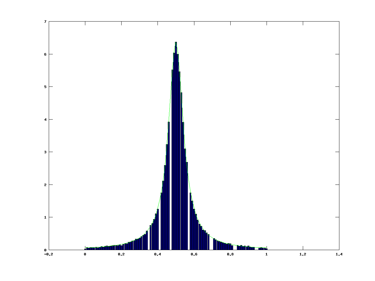
With this number of samples we get a much better resolution. We are easily able to make out the details of the curve. This is a good approximation of the function. If we were to see just the bars, we could quite easily work out what it was trying to represent. This is because the Monte Carlo method, combined with the law of large numbers, converges onto the true value of what you’re trying to represent. At  we would converge to a perfect Lorentzian. The gaps in the continuum are due to the random number generator, combined with the binning interval I used for the demonstration. The quality of the approximation can also be improved by improving the resolution of the binning.
This demo was inspired by this video by Steve Spicklemire. I highly recommend watching it if you’re interested. It really helped me understand some of the mathematics at work here.
Example: Calculating Pi
Here’s a really cool, if a little useless, example of how Monte Carlo methods can be used to solve realistic problems. In this case, we’ll be calculating the value of  . We can do this pretty easily using Monte Carlo Integration. This involves using a shape that you can easily calculate the area of, such as a square in the case of this example, and use the ratio of the number of points randomly distributed within both regions to calculate the area of the more complex shape, such as a circle. Mathematically, this is expressed like this
![\[\rho = \frac{\textrm{Area of Circle}}{\textrm{Area of Square}} = \frac{\pi r^2}{(2r)^2} = \frac{pi}{4}\]](https://sammorrell.co.uk/wp-content/ql-cache/quicklatex.com-4b5f1a9e4587a6d97180d6f7c1c79434_l3.png "Rendered by QuickLaTeX.com")
We can use this to help us out. By using the Monte Carlo method, we can place points randomly within the square and if they fall within the constrain of  then the point is within the circle. We can count up the number of point inside the circle and then the number of points inside the square (which should be all of them). By dividing these two number and multiplying by 4, due to the equation above, we will get a Monte Carlo approximation of
  . Enough chatting, let me give you a practical example.
In this simulation we used 10,000 total points placed at random in a 1×1 graph. Of that 10,000, 7854 of them ended up inside the region that denotes the circle. You can see an illustration of this below.

The ratios of these numbers of points can let us calculate the value of pi, like this.
![\[ \frac{7854}{10000} \times 4 = 3.1416 \]](https://sammorrell.co.uk/wp-content/ql-cache/quicklatex.com-ef3b21eada18fef2307abd4666e3cd9e_l3.png "Rendered by QuickLaTeX.com")
This was a good run, but given the number of points that you use the value attained can vary considerably. There are a couple ways to refine your answer. You can either increase the number of points that you’re placing in each simulation (which I found that both Octave and gnuplot don’t like an awful lot) or you can repeat the simulation and calculate the average of all these repetitions. Either way, there is one simple truth. The more samples you collect, the value that the simulation is providing you is converging on the true value of . I’ve included a link below to a piece by John H. Matthews and Kurtis Fink that is very good at describing this demo and more. It gives a few nice examples that should help if, like me, you have a little problem understanding on first glance.
http://math.fullerton.edu/mathews/n2003/montecarlopimod.html
Practical Monte Carlo
All this stuff is very useful, but up until this point I’ve not covered anything particularly ground breaking or even particularly useful. This brings me on to how physicists, in this particular situation astrophysicists, use the Monte Carlo method to solve real, practical problems such as the radiative transfer problem. As I said at the start, radiative transfer is the term used to describe the transfer of energy using photons. There is a very good description of the whole process here, written by Duncan Forgan of the Royal Observatory Edinburgh, but I’ll do my best to give a simplified explanation. The basics of this method is that we can do the same as we did in the first demonstration. By firing random values at some kind of probability distribution function (PDF), we can sample it. The distribution in this case is the emission spectra of a luminous stellar object, such as a star. By repeating the experiment above, we can construct a cumulative distribution function (CDF) where each value of Y between 0 and 1 maps uniquely onto a single value of X. The value of X in this case is the wavelength of our emitted photon. This works for stars, as more luminous areas of the spectrum will have a higher probability of emitting a photon of that wavelength. We now have the wavelength of our photon, now we need to decide where it’s going to go. We can do this once again by randomly sampling a function. In this case it’s a scattering probability function. Generally speaking, we can use ‘isotropic scattering’ which means that the photon has an equal probability of scattering in any direction. For the most simple version of the method, this is true for all processes that happen during the simulation; however this is mostly physically unrealistic and other, more complex methods have to be used for scattering. Before we can scatter the photon we have to work out where it’s going to scatter. To do this we calculate the mean free path of the photon. From this we can show that the PDF of a scattering event happening at optical depth  is
is
![\[ P(\tau) = 1 - e^{-\tau} \]](https://sammorrell.co.uk/wp-content/ql-cache/quicklatex.com-e57618d6a71b7bccb12808c8d75b17e3_l3.png "Rendered by QuickLaTeX.com")
If we invert this by making  the subject and making
  a random number, we have ourselves another out of the box use of the Monte Carlo method. When the photon reaches this point it can either scatter off the medium or be absorbed by the medium. This is determined once again by plugging random numbers into the albedo (the probability that the photon is scattered rather than absorbed) and phase function (the probability that the photon will be scattered by angle
  ) of the medium. It’s also at this point any computation specific to the simulation may happen, such as transferring energy to the medium from the photon of you were modelling radiative hydrodynamics; which is where the energy from radiation fields such as light cause a transfer of momentum or energy during an emission, scattering or absorption process, thus influence the outcome if we’re modelling the movement of the gases. We repeat this process, scattering or absorbing the photon until it leaves the grid that we are studying. At this point we look and see if it hits our imaging plane. If it does, we can treat it like any photon hitting a CCD (charge-coupled device) and register a count. After this we emit another photon and keep repeating this process until we begin to see a pattern building up on out imaging sensor. Low and behold, the mass amounts of random numbers we plugged into CDFs has given us a realistic, physically correct (well, as far as the simulation anyway) image of the system we are studying. If enough photons have been passed through the system (generally about 10s of millions depending on the simulation) we get a very low noise image that we can then study as if it were a real astronomical observation.
I’ve been working with the Torus radiative transfer code written by Professor Tim Harries of the University of Exeter. If you’re looking to try out a fully featured radiative transfer code, check out Torus Homepage, as I believe they’re heading for a public release fairly soon.
I hope this has been interesting. I know it has been for me. If there is anything that is out and out wrong and needs to be corrected, just let me know; after all the whole point of science if making mistakes, then you learn from them. If you have been, thanks for reading.
